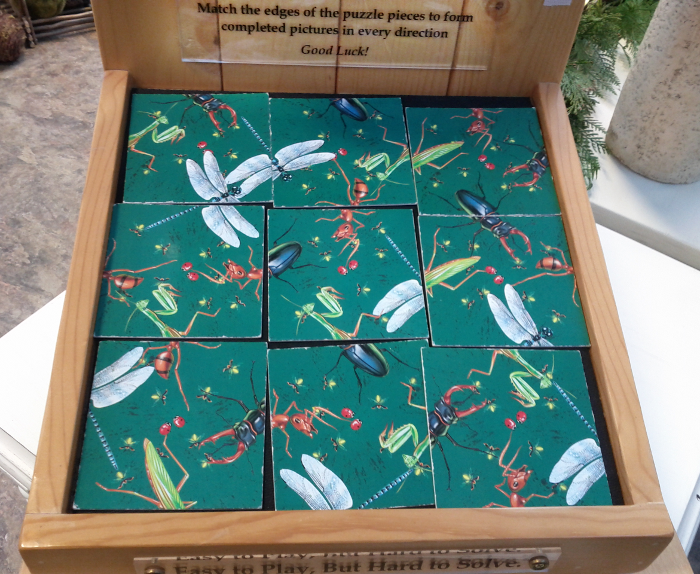
 The puzzle consists of nine square titles. The tiles must be placed so the pictures match up where two tiles meet. As the picture says, "Easy to play, but hard to solve." It turns out that this type of puzzle is called an edge-matching puzzle, and is NP-complete in general. For dozens of examples of these puzzles, see Rob's Puzzle Page.
Backtracking is a standard AI technique to find a solution to a problem step by step. If you reach a point where a solution is impossible, you backtrack a step and try the next possibility. Eventually, you will find all possible solutions. Backtracking is more efficient than brute-force testing of all possible solutions because you abandon unfruitful paths quickly.
To solve the puzzle by backtracking, we put down the first tile in the upper left. We then try a second tile in the upper middle. If it matches, we put it there. Then we try a third tile in the upper right. If it matches, we put it there. The process continues until a tile doesn't match, and then the algorithm backtracks. For instance, if the third tile doesn't match, we try a different third tile and continue. Eventually, after trying all possible third tiles, we backtrack and try a different second tile. And after trying all possible second tiles, we'll backtrack and try a new first tile. Thus, the algorithm will reach all possible solutions, but avoids investigating arrangements that can't possibly work.
The implementation
I represent each tile with four numbers indicating the pictures on each side. I give a praying mantis the number 1, a beetle 2, a dragonfly 3, and an ant 4. For the tail of the insect, I give it a negative value. Each tile is then a list of (top left right bottom). For instance, the upper-left tile is (2 1 -3 3). With this representation, tiles match if the value on one edge is the negative of the value on the other edge. I can then implement the list of tiles:
(with (mantis 1 beetle 2 dragonfly 3 ant 4)
  (= tiles (list
    (list beetle mantis (- dragonfly) dragonfly)
    (list (- beetle) dragonfly mantis (- ant))
    (list ant (- mantis) beetle (- beetle))
    (list (- dragonfly) (- ant) ant mantis)
    (list ant (- beetle) (- dragonfly) mantis)
    (list beetle (- mantis) (- ant) dragonfly)
    (list (- ant) (- dragonfly) beetle (- mantis))
    (list (- beetle) ant mantis (- dragonfly))
    (list mantis beetle (- dragonfly) ant))))
Next, I create some helper functions to access the edges of a tile, convert the integer to a string, and to prettyprint the tiles.
;; Return top/left/right/bottom entries of a tile
(def top (l) (l 0))
(def left (l) (l 1))
(def right (l) (l 2))
(def bottom (l) (l 3))

;; Convert an integer tile value to a displayable value
(def label (val)
  ((list "-ant" "-dgn" "-btl" "-man" "" " man" " btl" " dgn" " ant")
   (+ val 4)))

;; Print the tiles nicely
(def prettyprint (tiles (o w 3) (o h 3))
  (for y 0 (- h 1)
    (for part 0 4
      (for x 0 (- w 1)
        (withs (n (+ x (* y w)) tile (tiles n))
          (if
     (is part 0)
       (pr " ------------- ")
     (is part 1)
       (pr "|    " (label (top tile)) "     |")
     (is part 2)
       (pr "|" (label (left tile)) "    " (label (right tile)) " |")
     (is part 3)
       (pr "|    " (label (bottom tile)) "     |")
     (is part 4)
       (pr " ------------- "))))
      (prn))))
The prettyprint function uses optional arguments for width and height: (o w 3). This sets the width and height to 3 by default but allows it to be modified if desired. The part loop prints each tile row is printed as five lines. Now we can print out the starting tile set and verify that it matches the picture. I'll admit it's not extremely pretty, but it gets the job done:
arc> (prettyprint tiles)
 -------------  -------------  -------------
|     btl     ||    -btl     ||     ant     |
| man    -dgn || dgn     man ||-man     btl |
|     dgn     ||    -ant     ||    -btl     |
 -------------  -------------  -------------
 -------------  -------------  -------------
|    -dgn     ||     ant     ||     btl     |
|-ant     ant ||-btl    -dgn ||-man    -ant |
|     man     ||     man     ||     dgn     |
 -------------  -------------  -------------
 -------------  -------------  -------------
|    -ant     ||    -btl     ||     man     |
|-dgn     btl || ant     man || btl    -dgn |
|    -man     ||    -dgn     ||     ant     |
 -------------  -------------  -------------
Next is the meat of the solver. The first function is matches, which takes a grid of already-positioned tiles and a new tile, and tests if a particular edge of the new tile matches the existing tiles. (The grid is represented simply as a list of the tiles that have been put down so far.) This function is where all the annoying special cases get handled. First, the new tile may be along an edge, so there is nothing to match against. Second, the grid may not be filled in far enough for there to be anything to match against. Finally, if there is a grid tile to match against, and the value there is the negative of the new tile's value, then it matches. One interesting aspect of this function is that functions are passed in to it to select which edges (top/bottom/left/right) to match.
;; Test if one edge of a tile will fit into a grid of placed tiles successfully
;;  grid is the grid of placed tiles as a list of tiles e.g. ((1 3 4 2) nil (-1 2 -1 1) ...)
;;  gridedge is the edge of the grid cell to match (top/bottom/left/right)
;;  gridx is the x coordinate of the grid tile
;;  gridy is the y coordinate of the grid tile
;;  newedge is the edge of the new tile to match (top/bottom/left/right)
;;  newtile is the new tile e.g. (1 2 -1 -3)
;;  w is the width of the grid
;;  h is the height of the grid
(def matches (grid gridedge gridx gridy newedge newtile w h)
  (let n (+ gridx (* gridy w))
    (or
      (< gridx 0) ; nothing to left of tile to match, so matches by default
      (< gridy 0) ; tile is at top of grid, so matches
      (>= gridx w) ; tile is at right of grid, so matches
      (>= gridy h) ; tile is at bottom of grid, so matches
      (>= n (len grid)) ; beyond grid of tiles, so matches
      (no (grid n)) ; no tile placed in the grid at that position
      ; Finally, compare the two edges which should be opposite values
      (is (- (gridedge (grid n))) (newedge newtile)))))
With that method implemented, it's easy to test if a new tile will fit into the grid. We simply test that all four edges match against the existing grid. We don't need to worry about the edges of the puzzle, because the previous method handles them:
;; Test if a tile will fit into a grid of placed tiles successfully
;;   grid is the grid of tiles
;;   newtile is the tile to place into the grid
;;   (x, y) is the position to place the tile
(def is_okay (grid newtile x y w h)
    (and
      (matches grid right (- x 1) y left newtile w h)
      (matches grid left (+ x 1) y right newtile w h)
      (matches grid top x (+ y 1) bottom newtile w h)
      (matches grid bottom x (- y 1) top newtile w h)))
Now we can implement the actual solver. The functions solve1 and try recursively call each other. solve1 calls try with each candidate tile in each possible orientation. If the tile fits, try updates the grid of placed tiles and calls solve1 to continue solving. Otherwise, the algorithm backtracks and solve1 tries the next possible tile. My main problem was accumulating all the solutions properly; on my first try, the solutions were wrapped in 9 layers of parentheses! One other thing to note is the conversion from a linear (0-8) position to an x/y grid position.
A couple refactorings are left as an exercise to the reader. The code to try all four rotations of the tile is a bit repetitive and could probably be cleaned up. More interesting would be to turn the backtracking solver into a general solver, with the puzzle just one instance of a problem.
;; grid is a list of tiles already placed
;; candidates is a list of tiles yet to be placed
;; nextpos is the next position to place a tile (0 to 8)
;; w and h are the dimensions of the puzzle
(def solve1 (grid candidates nextpos w h)
  (if
    (no candidates)
      (list grid) ; Success!
    (mappend idfn (accum addfn ; Collect results and flatten
      (each candidate candidates
        (addfn (try grid candidate (rem candidate candidates) nextpos w h))
        (addfn (try grid (rotate candidate) (rem candidate candidates) nextpos w h))
        (addfn (try grid (rotate (rotate candidate)) (rem candidate candidates) nextpos w h))
        (addfn (try grid (rotate (rotate (rotate candidate))) (rem candidate candidates) nextpos w h)))))))

; Helper to append elt to list
(def append (lst elt) (join lst (list elt)))

;; Try adding a candidate tile to the grid, and recurse if successful.
;; grid is a list of tiles already placed
;; candidate is the tile we are trying
;; candidates is a list of tiles yet to be placed (excluding candidate)
;; nextpos is the next position to place a tile (0 to 8)
;; w and h are the dimensions of the puzzle
(def try (grid candidate candidates nextpos w h)
  (if (is_okay grid candidate (mod nextpos w) (trunc (/ nextpos w)) w h)
    (solve1 (append grid candidate) candidates (+ nextpos 1) w h)))
The final step is a wrapper function to initialize the grid:
(def solve (tiles (o w 3) (o h 3))
  (solve1 nil tiles 0 w h))
With all these pieces, we can finally solve the problem, and obtain four solutions (just rotations of one solution):
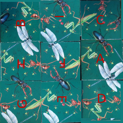
arc> (solve tiles)
(((1 -2 -4 3) (2 4 1 -3) (4 -1 2 -2) (-3 1 4 -2) (3 -4 -1 2) (2 1 -3 3) (2 -4 -1 -3) (-2 1 4 -3) (-3 -4 4 1))
((2 4 -2 -1) (-3 2 3 1) (4 -3 1 -4) (1 2 -3 4) (-1 3 2 -4) (4 -2 -3 1) (-4 1 3 -2) (4 -3 -2 1) (-1 2 -3 -4))
((1 4 -4 -3) (-3 4 1 -2) (-3 -1 -4 2) (3 -3 1 2) (2 -1 -4 3) (-2 4 1 -3) (-2 2 -1 4) (-3 1 4 2) (3 -4 -2 1))
((-4 -3 2 -1) (1 -2 -3 4) (-2 3 1 -4) (1 -3 -2 4) (-4 2 3 -1) (4 -3 2 1) (-4 1 -3 4) (1 3 2 -3) (-1 -2 4 2)))
arc> (prettyprint (that 0))
 -------------  -------------  -------------
|     man     ||     btl     ||     ant     |
|-btl    -ant || ant     man ||-man     btl |
|     dgn     ||    -dgn     ||    -btl     |
 -------------  -------------  -------------
 -------------  -------------  -------------
|    -dgn     ||     dgn     ||     btl     |
| man     ant ||-ant    -man || man    -dgn |
|    -btl     ||     btl     ||     dgn     |
 -------------  -------------  -------------
 -------------  -------------  -------------
|     btl     ||    -btl     ||    -dgn     |
|-ant    -man || man     ant ||-ant     ant |
|    -dgn     ||    -dgn     ||     man     |
 -------------  -------------  -------------
I've used gimp on the original image to display the solution. I've labeled the original tiles A-I so you can see how the solution relates to the original image. Using Arc to display a solution as an image is left as an exercise to the reader :-) But seriously, this is where using a language with extensive libraries would be beneficial, such as Python's PIL imaging library.
Theoretical analysis
I'll take a quick look at the theory of the puzzle. The tiles can be placed in 9! (9 factorial) different locations, and each tile can be oriented 4 ways, for a total of 9! * 4^9 possible arrangements of the tiles, which is about 95 billion combinations. Clearly this puzzle is hard to solve by randomly trying tiles.arc> (* (apply * (range 1 9)) (expt 4 9)) 95126814720
We can do a back of the envelope calculation to see how many solutions we can expect. If you put the tiles down randomly, there are 12 edge constraints that must be satisfied. Since only one of the 8 possibilities matches, the chance of all the edges matching randomly is 1 in 8^12 or 68719476736. Dividing this into the 95 billion possible arrangements yields 1.38 solutions for an arbitrary random puzzle. (If this number were very large, then it would be hard to create a puzzle with only one solution.)
We can test this calculation experimentally by seeing how many solutions there are are for a random puzzle. First we make a function to create a random puzzle, consisting of 9 tiles, each with 4 random values. Then we solve 100 of these:
arc> (def randtiles ()
  (n-of 9 (n-of 4 (rand-elt '(1 2 3 4 -1 -2 -3 -4)))))
arc> (n-of 100 (len (solve (randtiles))))
(0 0 0 8 0 0 0 8 0 0 0 0 0 0 0 0 0 0 0 4 0 0 0 0 0 0 0 0 0 0 8 0 0 4 0
0 0 4 8 0 8 0 0 0 0 0 0 0 32 0 0 0 0 0 0 0 0 0 0 0 0 0 0 0 0 0 0 16 0
0 0 32 8 0 0 0 0 0 0 0 0 12 0 0 0 0 0 0 0 0 0 0 0 8 0 0 4 0 0 32)
arc> (apply + that)
196
Out of 100 random puzzles, there are 196 solutions, which is close to the 1.38 solutions per puzzle estimate above. (
that is an obscure Arc variable that refers to the previous result.) Note that only 16% of the puzzles have solutions, though. Part of the explanation is that solutions always come in groups of 4, since the entire puzzle can be rotated 90 degrees into four different orientations. Solving 100 puzzles took 146 seconds, by the way.
Another interesting experiment is to add a counter to try to see how many tile combinations the solver actually tries. The result is 66384, which is much smaller than the 95 billion potential possibilities. This suggests that the puzzle is solvable manually by trial-and-error with backtracking; at a second per tile, it would probably take you 4.6 hours to get the first solution.
1 comment:
Can this work with puzzles that have to match two of the same colour together, for example red must be touching red?
Post a Comment