JavaScript secrets of Bret Victor's homepage

I recently came across the site worrydream.com, which implements an amazing navigation experience through JavaScript and HTML5. The page displays dozens of page icons arranged into angled strips that fit the page, and when you click on one, the icons fly around the page while the clicked link slides in at the bottom. It's an amazing effect - if you haven't seen the site, click on the image below to try it. (Otherwise this article won't make much sense.)

Looking at the page, I couldn't figure out how CSS and JavaScript could perform the effects on the page - the way the icons moved around, the angles of the icons and the page, or the way the page blurred and appeared. Using Inspect Element in the browser showed a whole bunch of complex divs, but didn't give much clue as to how it works.

I set out to understand in detail how the page works. In the process, I learned a lot of interesting JavaScript and CSS techniques, and I'll share them with you in this article.

So how does the page work?

If you do "View Source" on worrydream.com, you may be surprised - the page is mostly just a bunch of lists of text and links. In fact, if you use Internet Explorer, that's all you'll see - just a 1990's-era list of links. The following snippet shows part of the HTML source, which consists simply of a list of text and links. The HTML doesn't even contain images. The horizontal strips of icons aren't implemented anywhere in the source. So where does the page content come from?

<h2>Dynamic Pictures</h2>

<ul>

<li class="pageWidth-1070 subtitleOnly-1"><a id="DynamicPicturesMotivation" href="http://worrydream.com/DynamicPicturesMotivation/">

<span class="title">Dynamic Pictures</span></a>:

<span class="subtitle">Why do we make pictures by writing code? How can artists draw data graphics, visual interfaces, and other

<b>pictures that change</b>?</span>

</li>

<li class="pageWidth-1150 noPreload-1"><a id="MagicInk" href="http://worrydream.com/MagicInk/>

<span class="title">Magic Ink</span></a>:

<span class="subtitle">A treatise on a new approach to UI design. Interaction considered harmful.</span>

</li>

<li class="pageWidth-920"><a id="Substroke" href="http://worrydream.com/substroke/">

<span class="title">Substroke</span></a>:

<span class="subtitle">Sketch of a dynamic drawing language.</span>

</li>

</ul>

Generating totally new content from the existing page

It turns out that the JavaScript entirely hides the existing page content (by setting display: none on the top-level div) and dynamically generates totally new page content, which is what you see.

The following image shows the part of the page that is generated by the above HTML snippet. You can see a clear mapping from the headings and links in the source above to the text and icons in the image below, but this is all dynamically synthesized. That is, the JavaScript goes through the existing page and for each heading, list item, link, etc, it generates a bunch of entirely new elements. The source above is not rendered at all.

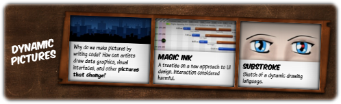
Note that the text in the HTML is displayed below the icons. In addition, the images are not explicitly specified in the HTML, but come from the id attributes, which I explain in more detail below. I also explain later how the class attributes work.

Most web pages use CSS to style the HTML content of the page with the desired page formatting and layout. Worrydream.com uses a very different approach where the existing page contents is input used to generate entirely new page content. This is one of the most interesting techniques of worrydream.com. It's even more impressive that the "template" content renders nicely as a fallback mechanism for Internet Explorer and other unsupported browsers.

The page implements many different JavaScript objects

The site is implemented with thousands of lines of JavaScript, and the scripts can be viewed here. The page is implemented from many different sub-components, each with complex behavior. A quick overview of these objects will help explain how the page is created.

The Site object is the key object that does most of the work. The main logic in Site scans through the divs in the original document and creates a SiteSection and SiteSectionTitleSet for each div. SiteSection in turn extracts the h2 and ul tags from the original page, creates a SiteStripSegment for each one, and lays them out on the page into a collection of SiteStrips. The Site object also creates many relatively minor components: SiteBackground for the page background, SiteContactSet for the sharing links, SiteDoodle for thie images at the top, SiteHomeButton, shadows, SitePageArrowRegion for the left and right buttons, and the custom scrollbars SiteXScroller and SiteYScroller.

The page format explodes dramatically when an icon is clicked

When an icon is clicked, the whole format of the page changes and the page components fly around in a dramatic way, seemingly exploding randomly. It is hard at first to follow what happens to all the icons when the page rearranges. In fact, the behavior is simpler than it seems. The new icon layout consists of a very long linear layout at the top of the screen, with most of the icons either off the left or the right of the screen. If you watch carefully, you can see the icons move into their new positions. Clicking the SiteHomeButton in the upper left reverses this movement. The diagram below shows that many new objects are used to display the page. The most important change is that the ContentContainer displays the page corresponding to the clicked icon.

The SitePageSet becomes visible after an icon is clicked. The SitePageSet manages the blurred page images, most of which extend off to the left and right of the visible screen. To initialize it, SiteSection added a SitePage to the SitePageSet for each element that it processed.

The ContentContainer holds the actual page contents when an icon is clicked. When I first looked at the site, I figured "Oh, the page you click on is loaded into an iframe." It turns out the site is considerably more complex. Simple pages are loaded into an iframe but there is special logic do display Vimeo, movies, images, or embedded HTML.

Pre-computed thumbnails and page images

One of the most dramatic elements of the page occurs when you click an icon - a blurred version of the page slides in and then jumps into focus. You might wonder what CSS trick creates the blurred page. The blurring turns out to be entirely precomputed - there is a small blurred snapshot of each page in a page image directory and that snapshot simply gets displayed while the real page is loading.

Similarly, all the page icons are stored in a thumbnail directory. Interestingly, the page images and icon images do not explicitly appear in the source, but are dynamically created. The id attribute on each link is used to generate the URLs. For instance a link with id="ScrollTabs" corresponds to images named ScrollTabs.jpg in the PageImages and ThumbnailImages directories.

The two lessons are: first, sometimes it's better to use an offline brute-force solution such as precomputing blurred images for every page, rather than trying to do it dynamically. And second, you can use a naming system to generate image links, rather than hardcoding them.

Details and techniques used by the site

The above explanation covers the high-level components of worrydream.com. The remainder will describe some of the interesting low-level functionality, implementation, and CSS tricks.

BVLayer library

The worrydream.com site is based on a "layer" abstraction, which is implemented through the BVLayer library. Layers can be considered as displayable objects implemented in JavaScript, with complex logic to control their appearance and behavior. Layers form a hierarchy, with layers containing other layers. If you look at the above diagrams, the components (SiteSection, SiteStripSegment, etc) are layers.

Each layer is implemented as a div, normally with another BVLayer div as a parent. This explains why looking at the page structure with Inspect Element just shows a huge number of divs.

Most of the JavaScript objects in worrydream.com are subclasses of BVLayer, with additional functionality implemented in the subclass. For some objects, this additional functionality is just a background image or an event handler, while other objects may be extremely complex, for instance Site, which hold the top-level logic for the page, or SiteSection, which has the layout engine for the page.

The library is complex - almost 1000 lines of JavaScript, and provides many functions. It provides a system to transform layers by moving or rotating them, as well as implementing animation. It includes a framework to handle mouse and touchpad events and provides browser-independent abstractions.

The touch events API

Many browsers now support a touch events API for use with touch-screen devices. These events are similar to the old mouse events such as mousedown, mouseup, but are modified to handle touch-screen characteristics such as multi-touch and pressure. The specific events are touchstart, touchend, touchenter, touchleave, and touchcancel. These events allow JavaScript applications to work in a natural way with touch-screen devices.

Worrydream.com makes heavy use of touch events. The BVLayer library builds an event system on top of mouse and touch events to detect movements, taps, double taps, and to implement touchable regions. This allows the site to support complex interations both on desktop and touch devices.

Web fonts

Much of the character of worrydream.com comes from its unusual display font. The website uses Komika fonts from FontSquirrel. These fonts are used through the CSS3 @font-face feature.

The web fonts feature allows a website to download desired fonts, rather than being limited to the standard browser fonts. A simple explanation of @font-face is here or you can read the official W3C CSS Fonts document. Web fonts can be obtained from a variety of sources, such as Google web fonts, Typekit, or Fonts.com.

MooTools

The worrydream.com site is implemented using MooTools, which is apparently the second-most popular JavaScript framework/library after jQuery. The main distinguishing feature of MooTools is it provides a standard Object-Oriented class model with inheritance, rather than the prototype-based inheritance of JavaScript. MooTools also provides browser-independent JavaScript tools for accessing the DOM, handling events, performing animations, Ajax operations, and other standard JavaScript library features.

The worrydream.com website makes heavy use of MooTools, but builds complex layers of abstraction on top of it.

More information on MooTools is available at MooTools.net, Wikipedia, the MooTorial tutorial site, or books such as MooTools 1.2 Beginner's Guide.

Object parameters come from the CSS class names

If you look at the CSS classes in the HTML source, you see interesting class names such as

<li class="pageColor-0c0c0c pageWidth-900 pageHeight-970 injectContent-1">

Surely there's not a separate CSS class defined for each page color, witdth, and height?

The worrydream.com code uses an interesting properties system (see Site.mergePropertiesFromElement) to turn the "classnames" into object properties. This function parses each hyphen-separated entry in the class attribute, so the above would generate the properties {pageColor: "0c0c0c", pageWidth: 900, pageHeight: 970, injectContent: 1}. These properties are then used to control the new elements that get created on the page.

The properties system provides a few additional features. For instance, it supports string, integer, and percent types - scalePercent-68 turns into {scale: 0.68}. It also allows properties to be inherited from other elements.

This class-based property system is a clever way to pass arbitrary parameters into the page-generation system, while causing these parameters to be ignored by browsers that are rendering the original page. There are over 30 different properties used to change the rendering style for particular sections (filmEdges-1 to give the top strip film-style edges), specify special content (vimeo-23839605 to load a Vimeo video), provide special behavior (magicSubtitle-1 to enable the Easter Egg), specify dimensions (pageWidth-960), and many other functions.

Special support for Ajax URLs

You may notice that as you click on different icons, the URL changes to something like http://worrydream.com/#!/KillMath. Why the strange #! in the URL?

This style of URL is a standard technique for dynamic pages, allowing the use of the back arrow, bookmarks, and sharing links. Normally, if you change a page's URL via JavaScript, the entire page will reload, which is generally undesirable for a dynamic site. However, everything after the pound sign is a URL fragment identifier, which can be modified without reloads. Dynamic pages take advantage of this - they can update the fragment identifier in the URL to reflect page state, without triggering a disruptive page load. The second aspect of fragments in dynamic pages is if the anchor is changed (either by the user including the anchor in a URL or by the back arrow), the JavaScript must update the page to display the "right" content for that anchor.

But what is the exclamation point doing in there? This enables web crawlers to crawl the content, using an Ajax crawling standard. This allows Web crawlers to get the HTML page contents without needing to execute the JavaScript.

This Ajax crawling technique is important for any site that dynamically generates pages with JavaScript and wants the pages to get rendered properly by web crawlers.

CSS transformations

One of the most eye-catching effects on worrydream.com is that most of the elements on the page are arranged at slight angles, rather than the normal grid. This is implemented through CSS transformations, and the BVLayer library provides suport for these operations on any of the layers.

Most modern browsers support 2D transforms through CSS, allowing an element to translate(), rotate(), scale(), skew(), or be transformed through an arbitrary matrix(). (spec) This can be done easily in CSS, for example:

-webkit-transform: rotate(5deg);

Inconveniently, "webkit" must be replaced by "ms", "o", or "moz", depending on the browser type. The BVLayer library provides a browser-independence layer that hides that complication.

Animation through CSS transitions

The most eye-catching part of the site is how parts of the page fly around. This is implemented through CSS transitions and animations. CSS animations are supported by many browsers, and provide an easy way to animate to perform various animations. (spec)

Transitions can be implemented by setting a duration:

-webkit-transition-duration: 1s;

The BVLibrary handles multiple browsers, abstracting out the browser-specific prefixes such as -webkit- or -ms-, and providing fallbacks for less capable browsers. For instance, if the browser doesn't support transitions, the library uses the MooTools Fx.Tween method to perform the animations.

Hardware Acceleration

One trick I learned from the code is that the translate3D() CSS property will enable hardware acceleration on iOS. This lets the site work more smoothly on these devices.

Attention to detail

One surprising thing about worrydream.com is the attention to detail. Whenever I think something has an obvious implementation, it turns out to have additional complexity. For instance, the cannon and windmill images at the top of the page are not just images, but two SiteDoodle classes, which contain animation logic and fade-out logic that is activated when the page changes.

Another hidden feature is the "Easter Egg" that is activated when clicking on the "purveyor of impossible dreams" subtitle at the top of the page. Its implementation is a significant amount of code, but I'll leave the details as a surprise.

The scrollbars at the top and right of the page are not standard browser scrollbars, but custom-implemented scrollbars with their own styling and logic.

The Twitter, RSS, and email icons at the top of the page are not simply icons, but SiteContactSet and SiteContact classes with their own logic, as well as separate implementations for the bottom of the page.

The page background is not just a simple background, but a set of SiteBackground classes implemented from BVLayer. The shadows around the edges of the page are also implemented through BVLayer.

The page contains complex logic to lay out the icons according to the page dimensions and redo the layout if the browser is resized.

My conclusion is that a site like worrydream.com isn't made by simply adding some JavaScript functions to a page, but by implementing every aspect of it with careful attention to the details. I hate to imagine how much time it must have taken to implement the site.

Conclusions

I should re-emphasize that worrydream.com is not my site and I have no connection to it. I found it fascinating and asked its creator Bret Victor if I could study it and write about it. The site has many other pages that display interesting JavaScript techniques and are worthy of investigation, such as Scientific Computation, Ladder of Abstraction, Ten Brighter Ideas, and Explorable Explanations, but I don't have space to describe them here.

By examining the worrydream.com site in detail, I learned a lot about how to build a complex site out of JavaScript and take advantage of CSS3 functions. I hope that you have also learned some interesting techniques by reading this article.

A new multi-branch algorithm to render rational-exponent Mandelbrot fractals: Part I

If you came here from Hacker News, thanks for visiting. You might want to check out the Hacker News comment thread too.

The Mandelbrot fractal is generated by repeatedly iterating the complex function f(z) = z^2 + c, and testing if the result diverges to infinity or not. An obvious generalization is to use a different exponent in place of 2 (yielding a fractal sometimes called the Multibrot). In this article, I describe a new algorithm for fractals with a rational exponent, for example z^2.5+c. This algorithm uses all branches of the complex roots in parallel, rather than just the principal root, which displays new structure of the fractal.

Previous techniques to display fractional-exponent fractals force the multi-valued complex root to have a single value, which distorts the "true" fractal. By computing all the possible root values in parallel, I determine the "true" form of the fractal.

The following image shows the multi-branch fractal for z^2.5+c. Click on the image (or any of the other images) for a full-size version.

The multi-branch fractal for z^2.5+c.

The problem with square roots

Numbers generally have two square roots, although we typically only think about the principal (positive) one. For instance (-2)² = 2² = 4, so sqrt(4) = +2 or -2. (Zero is the exception.) Likewise, complex numbers have two square roots. Unfortunately, we can't just pick one of the square roots without running into discontinuities. For instance, suppose we start with sqrt(1) = 1. Then look at sqrt(i), sqrt(-1), and sqrt(-i) on the following diagram. The roots are nice and continuous from (A) to (D) until we end up back at (E), where sqrt(1) = -1. Something has to give; somewhere the square root function is going to become discontinuous.

This problem can be solved by making a branch cut, where the function is discontinuous. This cut is typically along the negative real axis, so at point (C) the square root function would jump from i to -i. Note that cutting along the negative real axis is arbitrary.

The disadvantage of making the square root function discontinuous is the resulting fractatals will have discontinuities. In addition, the appearance of the fractal will change if the arbitrary cut is made in a different location. Thus, in a sense, if you generate a fractal based on z^2.5+c, you're not seeing the real fractal, but artifacts based on arbitrary decisions.

Multi-valued complex functions can be expressed as Riemann surfaces. Instead of being defined on the complex plane, the function is defined on a surface which locally looks like the complex plane, but can have more structure. For instance, the following illustration shows the Riemann surface for the complex square root. Note that for each point (except 0), there are two values for the square root.

A Riemann surface for the complex function f(z) = sqrt(z).

ParametricPlot3D[{r * Cos[theta], r * Sin[theta], Sqrt[r] * Cos[theta/2]}, {theta, 0, 4Pi}, {r, 0, 5}, PlotPoints -> 100, PlotStyle->Opacity[.6], ViewPoint -> {-2, -2, 1}, Mesh->True, ColorFunctionScaling->False, ColorFunction -> Function[ {x,y,z,theta, r}, Hue[theta/(4Pi), .9, .9]]]

How do you compute a complex root?

In general, a complex power a^b is defined as exp(b * ln(a)), using the complex exponential and logarithm. The complex logarithm is multi-valued, which is the base of the multi-valued problems. These functions can be computed using well-known formulas.

Because I'm using square roots instead of arbitrary powers (for now), I can use a simpler complex square root formula (details at Wikipedia). The following code takes a complex number x + i * y, and returns the primary square root x1 + i * y1. Note that the negative -(x1 + i * y1) is the other square root.

public static void csqrt(double x, double y, ref double x1, ref double y1)
{
  double m = x * x + y * y;
  double r = Math.Sqrt(m);
  x1 = Math.Sqrt((r + x) / 2.0);
  if (y > 0) {
    y1 = Math.Sqrt((r - x) / 2.0);
  } else {
    y1 = -Math.Sqrt((r - x) / 2.0);
  }
}

Generating the real fractal, with all the branches

The key idea of the multi-branch algorithm is instead of forcing the square root function to have a single arbitrary value, embrace the multi-valued nature of the square root and try both values. In this way, we can see the "true" picture of the fractional-exponent Mandelbrot set. Specifically, instead of taking one value for the square root, the algorithm evaluates the fractal recursively trying each square root in turn. The two return values are combined to yield the final result.

To generate the multi-branch fractal, we can test each point to see if any branch converges. However, the result is more interesting if we count how many of the branches converge for each pixel. The result can be anywhere between all of them (in the middle of the fractal) to none of them (outside the fractal).

To decide if a point diverges, I use the standard escape-time technique of checking if the magnitude of z exceeds a bound. If z exceeds the bound, I know the point diverges. If z doesn't exceed the bound by the end of the iterations, I assume it doesn't diverge. This is not necessarily true, which is why the accuracy of a fractal increases as the number of iterations increases. I test for divergence with a bound of magnitude^2 > 4; the exact value of the bound doesn't make much difference as long as it is large enough to guarantee divergence.

The following code shows how the number of convergent branches c is computed recursively. Note that (z25x, z25y) is one of the values of z^2.5, and (-z25x, -z25y) is the other. The key to the multi-branch fractal is that both paths are explored, rather than just one. For a particular pixel, eval(x, y, x, y, 0) is called and the the result is displayed with a suitable colormap.

int eval(double zx, double zy, double cx, double cy, int n)
{
  if (n == max)
  {
    return 1;
  }
  // zsquared is z^2, zroot is sqrt(z), z25 is z^2.5
  double zsquaredx = zx * zx - zy * zy;
  double zsquaredy = 2 * zx * zy;
  double zrootx = 0, zrooty = 0;
  CMath.csqrt(zx, zy, ref zrootx, ref zrooty);
  double z25x = zsquaredx * zrootx - zsquaredy * zrooty;
  double z25y = zsquaredx * zrooty + zsquaredy * zrootx;

  int c = 0;
  // Use the first root
  double newx1 =  z25x + cx;
  double newy1 =  z25y + cy;
  if (newx1 * newx1 + newy1 * newy1 < 4)
  {
    c += eval(newx1, newy1, cx, cy, n + 1);
  }

  // Use the second root
  double newx2 = -z25x + cx;
  double newy2 = -z25y + cy;
  if (newx2 * newx2 + newy2 * newy2 < 4)
  {
    c += eval(newx2, newy2, cx, cy, n + 1);
  }
  return c;
}

The multi-branch fractal is exponentially slow compared to regular escape time fractals. At each iteration, there are two choices of square root, with the consequence that we evaluate 2^n values at each pixel, rather than n with a normal escape-time fractal. Unfortunately, this makes computation very expensive. For a regular escape-time fractal, you might use an iteration depth of hundreds for each pixel. But for the multi-branch fractal, it gets very slow if you go above about 12 iterations.

The above algorithm provides detail of the "inside" of the multi-branch fractal. Note that there is a central region where every branch converges. This isn't too surprising, since if c is sufficiently small, z^2.5 will converge with either branch. Outside this region is a complex area where points just barely converge on some branches, and flipping the branch anywhere will make the point diverge. The eight "snowflake" buds are what I find most interesting; these are regions that diverge for almost all branches, but converge for the "right" branches.

The resulting fractal is obviously symmetric when reflected in the y axis or when rotated by 60 degrees. The proofs are straightforward . In comparison, the regular z^2.5+c fractal is not rotationally symmetric because of the effect of branch cuts.

I believe the multi-branch fractal is connected (unlike the regular z^2.5+c fractal), but I don't have a proof. Interestingly, the fractal has some holes (i.e. is not simply connected). I believe these happen where different branches overlap in such a way that they happen to leave gaps, but on a particular branch (whatever that means) the fractal does not have holes.

The best way to see the holes is to look at the "outside" of the fractal. Instead of counting how many branches converge, the code can be easily modified to determine the maximum number of iterations it takes for a branch to diverge. This is similar to the standard escape-time fractal algorithm with level sets approaching the fractal (except of course, it uses multiple branches). In the image below, you can see dark blue spots inside the fractal near the "snowflakes" that look like image noise. These are actually areas that are outside the fractal with complex structure.

The multi-branch fractal for z^2.5+c, showing details of the exterior.

Stepping through iteration-by-iteration

One way to understand the multi-branch fractal is to step through one iteration at a time. If we start with one iteration, there are two branches at each pixel. We see a central region that converges for both branches, and three lobes that converge only for one branch. Note that the boundary wraps around the center twice. Perhaps you can imagine this boundary on the Riemann surface at the top of the page.

After two iterations, the structure is considerably more complex. Each point has four different branch possibilities, and can converge on 0 to 4 of the branches. The boundary now winds around 4 times on a more complex Riemann surface. Note that each boundary in the first image has split into two boundaries woven together - these are the two different branches for the second iteration.

With three iterations, the rough shape of the multi-branch fractal is starting to appear.

The multi-branch fractal for z^2.5+c, showing the number of convergent branches after 3 iterations.

Jumping to 14 iterations, the fractal has achieved its basic shape. Note the rough shape of the central region that converges for all branches. It is surrounded by many chaotic stripes, where most of the branches converge, but a few diverge. There are three big regions that mostly converge to two-cycles, and three smaller regions that mostly converge to three-cycles. The snowflakes, which diverge for almost all branches, are now clearly visible.

The multi-branch fractal for z^2.5+c, showing the number of convergent branches after 14 iterations.

Snowflakes and the Monkey's Paw

The "snowflakes" are made of a repeated motif that I call the "monkey's paw". Looking at one of these regions while increaing the number of iterations helps illustrate some of the structure of the fractal. After 3 iterations, a basic four-fingered "paw" is visible.

Multi-sheet z^2.5+c fractal at (-.90, 1.14): 3 iterations

After one more iteration, each finger splits into a new four-fingered paw. If you follow the edge of the paw, you'll discover a complex topology that winds through the paws in the order 2, 4, 1, 3, and winds through the fingers of each paw in the same order. This helps to illustrate the complex geometry of the underlying Riemann surface, which is splitting in the middle of each paw. (I hope to generate a 3D image to make this clearer.)

Multi-sheet z^2.5+c fractal at (-.90, 1.14): 4 iterations

After another iteration, each finger sprouts another new paw, and paws are starting to bud on the arms.

Multi-sheet z^2.5+c fractal at (-.90, 1.14): 5 iterations

After 6 iterations, there are paws sprouting everywhere. There is also a stable region in the middle of the original paw that converges for most of the branches.

Multi-sheet z^2.5+c fractal at (-.90, 1.14): 6 iterations

Finally, jumping to 12 iterations, the paws have developed into "snowflakes", with five-fold branching (the four fingers plus the arm). The five-fold branching appears all over the fractal. In the middle of each paw is a stable rgion, which is roughly self-similar to the overall fractal. (Just like tiny Mandelbrots appear in the threads of the Mandelbrot set.)

Multi-sheet z^2.5+c fractal at (-.90, 1.14): 12 iterations

Edge detection

Another way to see the structure is to filter the fractal to show the edges. This shows the structure of the boundary between convergent and divergent regions. The following image show the boundary after three iterations. If you follow the line around, you can see its complex structure.

Multi-sheet z^2.5+c fractal: edges of escape regions after 3 iterations.

After 5 iterations, the boundary has become very complex. Note the development of the "monkey's paws" discussed earlier. Also notice how many boundaries pass near the central region, causing the complexity there.

Multi-sheet z^2.5+c fractal: 5 iterations, edges of escape regions after 5 iterations.

Comparison with the "regular" escape-time fractal

Comparing the multi-branch fractal with the single-branch fractal shows some interesting features. The image below is the fractal generated from z^2.5+c using the standard algorithm. Superficially, it looks a lot like the Mandelbrot set. However, note that it is not connected, with some unconnected islands in the upper center for example.

The regular escape-time fractal for z^2.5+c.

Zooming in on one of the "antennas" of the regular fractal illustrates more of the disconnected components. You can also see the discontinuities due to the branch cut, lines where the fractal gets cut off. There is also a somewhat self-similar region, in yellow.

Regular escape-time fractal at (-.82, 1.21)

Below is the same region of the fractal, displayed using the multi-branch algorithm. Note that there is much more detail provided by the multi-branch algorithm. Also note that the stable self-similar region looks very much like the overall multi-branch fractcal.

Multi-branch fractal at (-.82, 1.21)

The regular fractal is actually a subset of the multi-branch fractal, since each computation in the single-branch fractal will be done in one of the paths of the multi-branch fractal. In the image below, the regular fractal has been overlayed on the multi-branch fractal. Note that the regular fractal exactly falls onto the multi-branch fractal, but is missing most of the branchess. Clicking on the image below will show an animation flipping between the regular fractal and the multi-branch fractal.

Overlay of regular escape-time and multi-branch fractals at (-.82, 1.21)

One surprising thing is how different the regular and multi-branch fractals look in general. The regular fractal looks much more "Mandelbrot-like" with its sequences of bulbs. I expect that the multi-branch fractal also has a similar structure, but hidden by the overlapping branches.

Another way of seeing how the fractals are related is to overlay the regular fractal with the edge map of the multi-branch fractal. In the following image, both fractals are rendered to a depth of 5 iterations. The regular fractal is displayed in cyan on top of the edges of the multi-branch fractal. Note that the edges match exactly, which is expected from the mathematics. Note also that the regular fractal jumps from curve to curve as it hits the branch cuts, rather than following a single curve. Also note how much of the multi-branch struture is missed by the regular fractal. (The regular fractal is very "blobby" because the iteration count is so low. A higher iteration could would make it too hard to see the edges.)

Multi-sheet z^2.5+c fractal: 5 iterations, edges of escape regions. Overlaid with regular z^2.5+c fractal.

What's next?

There are many more things to explore with multi-branch fractals. The techniques can easily be extended to values other than 2.5. Rendering Julia sets instead of Mandelbrot sets is straightforward, but I haven't looked into that yet; it's just a matter of fixing c and varying z, instead of varying z.

A more interesting exploration is looking at the fractal in three dimensions. In particular, I want to examine the Riemann surface structure in more detail. I think separating out the sheets of the surface will expose much more of the fractal structure, which gets hidden when all the sheets are projected together. I tried to compute the Riemann surface for just two iterations of a similar function using Mathematica but the result is almost incomprehensible:

Riemann surce of (z^2+.z)^.5
RiemannSurfacePlot3D[ w == (z^2.5+z)^.5, Re[w], {z, w}, PlotPoints -> {46, 44}, ImageSize -> 1260, Coloring -> Hue[Im[w]/8]]/. gc_GraphicsComplex :> {Opacity[0.66], gc} Multi-sheet z^2.5+c fractal at (-.90, 1.14): 5 iterations, edges of escape regions

An alternative way to compute the multi-branch fractal is to walk around the edge of the fractal. The result should be similar to the edge pictures above. However, walking pixel-by-pixel would have a few advantages. First, it would be much more efficient, allowing a much deeper iteration count which should show interesting fractal structure. Second, walking around only part of the edge will keep parts of the fractal from obscuring other parts.

I think the orbit behavior of individual starting points is a key to understanding this fractal. For instance, which starting points yield a 1-cycle, 2-cycle, and so forth. It's hard to define these cycles exactly, because of the multi-value nature of the fractal. A value can converge to a fixed point on one branch, but not another.

Another mathematical feature that I think is key to understanding the fractal is points where the value goes to zero. The function has many more zeros than I expected, and they are concentrated at "interesting" points of the fractal. The zeros are where the Riemann surfaces come together, and also the points where the boundary forms "loops".

I've been exploring different ways of displaying cycles and zeros, and hope to post images soon, but this post is already very long, so I'll leave those for Part II.

Related work

Many people have generated Mandelbrots with non-integer exponents, but always using a single-valued function. Wikipedia has a summary under the title Multibrot set.

I started investigating multi-branch fractional exponents many years ago but computers weren't powerful enough at the time, so my investigation didn't get very far. My negative integer exponents were easier to compute and I wrote a paper about those fractals: ``An Investigation of z -> 1/z^n+c,'' Computers & Graphics, 17(5), Sep. 1993, pp 603-607.

Joshua Sasmor has done an extensive investigation of non-integer exponents in his PhD thesis "Fatou, Julia and Mandelbrot Sets for Functions with Non-Integer Exponent" and in the paper "Fractals for functions with rational exponent", Computers and Graphics 28(4). Also of interest is his presentation Julia Set and Branch Cuts which shows the Julia set for z^2.5 - 1/2 + i/10 using inverse iteration instead of escape time. I suspect that his inverse iteration Julia set algorithm yields results similar to applying my multi-branch algorithm to Julia sets. I haven't explored this yet, but if true, it would provide more evidence that the multi-branch algorithm gives the "real" structure of the fratals.

There are several interesting videos that show the evolution of the generalized Mandelbrot set as the exponent changes. A few examples are Mandelbrot Set from 1 to 100 with zoom, Cut along negative X axis, and Cut along negative Y axis. It is interesting to compare the last two, to see how different the results are if the branch cut is placed in a different location.

Conclusion

The multi-branch algorithm provides an interesting new way to display Mandelbrot-like fractals that have non-integer exponents

Cells are very fast and crowded places

I recently learned that cells are extremely crowded and busy places. I knew there's a lot of activity in cells, but I didn't realize just how much until I was reading Molecular Biology of the Cell. I was reading this molecular biology textbook to find out what's happened in molecular biology in the last decade or so, and found I had some misconceptions about how fast things happen inside cells.

You may have seen the amazing "Inner Life of a Cell" video, which has spectacular animations of the activities inside a cell as a whilte blood cell responding to inflammation. (There's also a longer narrated version at the BioVisions website.)

Cells are very crowded

I imagined cells as big open spaces with lots of stuff happening, perhaps something like Central Park. From the "Inner Life of a Cell" video, or the typical drawing of a cell, it looks like a lot of empty space. But it turns out that cells are crammed full of stuff, more like New Year's Eve at Times Squares. Proteins are packed tightly into cells. The following picture is a representation of how crowded cells really are, with blue RNAs, green ribosomes, and red proteins.

Image: "The structure of the cytoplasm" from Molecular Biology of the Cell. Adapted from D.S. Goodsell, Trends Biochem. Sci. 16:203-206, 1991.

I came across another interesting representation of how crowded cells are. This diagram shows a synaptic vesicle, which is the part of a neuron that releases neurotransmitters from one neuron to another. When I saw this diagram, I assumed that the authors crammed all the different proteins into the picture so they could create a nice illustration of the different membrane proteins. But in fact, the diagram below omits 1/3 of the proteins so real membranes are even more crowded. The paper containing this diagram states that instead of thinking of membranes with proteins floating in them like icebergs, we should think of membranes as packed with proteins like a cobblestone pavement.

Image: "Molecular Model of an Average SV" from Molecular Anatomy of a Trafficking Organelle, Takamori et al, Cell. 2006 Nov 17;127(4):831-46.

Molecules move very very fast

You may wonder how things get around inside cells if they are so crowded. It turns out that molecules move unimaginably quickly due to thermal motion. A small molecule such as glucose is cruising around a cell at about 250 miles per hour, while a large protein molecule is moving at 20 miles per hour. Note that these are actual speeds inside the cell, not scaled-up speeds. I'm not talking about driving through a crowded Times Square at 20 miles per hour; to scale this would be more like driving through Times Square at 20 million miles per hour!

Because cells are so crowded, molecules can't get very far without colliding with something. In fact, a molecule will collide with something billions of times a second and bounce off in a different direction. Because of this, molecules are doing a random walk through the cell and diffusing all around. A small molecule can get from one side of a cell to the other in 1/5 of a second.

As a result of all this random motion, a typical enzyme can collide with something to react with 500,000 times every second. Watching the video, you might wonder how the different pieces just happen to move to the right place. In reality, they are covering so much ground in the cell so fast that they will be in the "right place" very frequently just by chance.

In addition, a typical protein is tumbling around, a million times per second. Imagine proteins crammed together, each rotating at 60 million RPM, with molecules slamming into them billions of times a second. This is what's going on inside a cell.

I'm not blaming the makers of "Inner Life of a Cell" for slowing down the action in a cell. If the video were totally realistic, you wouldn't see anything, since the action would be too fast to even see a blur. But keeping the real speed of the cell in mind can clear up a lot of things, such as how molecules find their way around.

The incredible speed and density of cells also helps explain why it's so difficult to simulate what's happening inside a cell. Even with a supercomputer, there's way too much going on inside a cell to simulate it without major simplifications. Even simulating a single ribosome is a huge computational challenge.

Molecular motors sprint, not walk

Another thing that surprised me about cells is how fast the motors inside cells move. Like a mechanical robot with two lumbering feet, a kinesin motor protein can be seen in the video at the 2 minute mark dragging a monstrous bag-like vesicle along a microtubule track. (This should be what you see in the YouTube preview frame at the top of the page.) These motor proteins move cargo through the cell if diffusion isn't fast enough to get things to their destination, which is especially important in extremely long cells such as neurons. Kinesin motors also help separate cells that are dividing.

It's remarkable enough that cells contain these mechanical walkers, but I recently learned that they aren't plodding along, but actually sprint at 100 steps per second. If you watch the video again, imagine it sped up to that rate.

Cells are powered by electric motors spinning at 40,000 rpm

Mitochondria also provide a fascinating look at just how fast things are inside cells. You may know that mitochondria are the power plants of cells; they take in food molecules, process it through the famous citric acid cycle, and then use oxygen to extract more energy, which is provided to the rest of the cell through molecules of ATP, the cell's "energy currency".

Image from David Goodsell, ATP Synthase, December 2005 Molecule of the Month

Mitochondria have many strange features - such as their own DNA separate from the cell's - but one of their strangest features is they use electric motors to produce ATP. Mitochondria use the energy from oxidizing food to pump protons out of the cell, creating a voltage of 170mV across the cell. This voltage causes a complex enzyme to spin, and the mechanical energy of this spinning enzyme creates the ATP molecules that energize the rest of the cell.

The same Harvard group that created "Inner Life of a Cell" also created a two minute sequel, "Powering the Cell: Mitochondria", which shows mitochondria in action. Around the 1:10 mark, the video shows the rotating ATP synthase enzymes creating glowing ATP molecules.

Watching the leisurely turning enzymes illustrates one of the amazingly complex mechanisms in a cell. But what really surprised me was to learn that in real life, these enzymes spin at up to 700 revolutions per second, which is faster than a jet engine. As I said earlier, cells are really, really fast.

If you're interested in more about this mechanical motor, you'll probably enjoy PDB's molecule of the month article.

Conclusions

The molecules inside a cell are moving almost unimaginably fast. Understanding this speed helped me comprehend how cells could carry out all their tasks, and how the different components of a cell could manage to be in the right place at the right time.

The BioVisions videos are very interesting, and I highly recommend watching them. (I also found Molecular Biology of the Cell very interesting and readable, but as it is a 1200+ page text, I don't imagine many people would read it unless they had to. But if you're still reading this article, maybe you're one of those people.)

The Mathematics of Volleyball

Recently I was at a multi-day volleyball tournament, which gave me plenty of time to ponder the mathematics of the game. At different points in the game, I'd wonder what the odds were of each team winning. And when a team gained or lost a point, I'd wonder how important that point was. Clearly, if the score was 24-24, gaining a point made a huge difference. But how much difference did getting one point at the beginning of the game matter? It seemed like it didn't matter much, but did it?

I decided to analyze the game mathematically. I made the simplifying assumption that each team had 50-50 odds of winning each point. I found the analysis interesting, and it turns out to have close ties to Pascal's Triangle, so I'm posting it here in case anyone else is interested.

Volleyball games are scored using the rally point system, which means that one team gets a point on every serve. (Back in the olden days, volleyball used side-out scoring, which meant that only the serving team could get a point. Fortunately, rally point scoring is more mathematically tractable. Rally point scoring also keeps the game advancing faster.) The winner of each match is the best out of three sets (a set is the same as a game). In the league I was watching, the winner of a game is the first team to get 25 points and be ahead by at least 2. (Except if a third tiebreaker game is needed, it only goes to 15 points instead of 25.)

A few cases are easy to analyze mathematically. If we assume each team has a 50-50 chance of scoring each point and the score is tied, each team obviously has a 50% chance of winning the game. (With side-out scoring, it makes a difference which team is serving, but for rally point scoring we avoid that complication.) The second obvious case is if a team has 25 points and the other team has 23 or fewer points, the first team has 100% chance of winning (since they already won).

I will use the notation P(m,n) for the chance of the first team wining if the score is m to n. From above, P(n, n) = 50%, P(25, n) = 100% for n <= 23, and P(m, 25) = 0% for m <= 23.

The chance of winning in other cases can be calculated from the assumption that a team has a 50% chance of winning the point, and a 50% chance of losing: the chance of winning is the average of these two circumstances. Mathematically, we get the simple recurrence:

For instance, if the score is 25-24, if the first team scores, they win. If the second team scores, then the score is tied. In the first (winning) case, the first team wins 100%, and in the second (tied) case, the first team wins 50%. Thus, on average they will win 75% of the time from a 25-24 lead. That is, P(25, 24) = 75%, and by symmetry P(24, 25) = 25%. (Surprisingly, these are the only scores where the requirement to win by 2 points changes the odds.)

Likewise, if the score is 24-23, half the time the first team will score a point and win, and half the time the second team will score a point and tie. So the first team has 1/2 * 100% + 1/2 * 50% = 75% chance of winning, and P(24, 23) = 75%.

More interesting is if the score is 24-22, half the time the first team will score a point and win, and half the time the second team will score, making the score 24-23. We know from above that the first team has a 75% chance of winning from 24-23, so P(24, 22) = 1/2 * 100% + 1/2 * 75% = 87.5%.

We can use the recurrence to work backwards and find the probability of winning from any score. The following table shows the probability of winning for each score. The first team has the score on the left, and the second team has the score on the top.

Table with odds of winning when the score is m to n

	0	1	2	3	4	5	6	7	8	9	10	11	12	13	14	15	16	17	18	19	20	21	22	23	24	25
0	50%	44%	39%	33%	28%	23%	18%	14%	11%	8%	5%	4%	2%	1%	1%	0%	0%	0%	0%	0%	0%	0%	0%	0%	0%	0%
1	56%	50%	44%	38%	33%	27%	22%	17%	13%	10%	7%	5%	3%	2%	1%	1%	0%	0%	0%	0%	0%	0%	0%	0%	0%	0%
2	61%	56%	50%	44%	38%	32%	27%	21%	17%	13%	9%	7%	4%	3%	2%	1%	1%	0%	0%	0%	0%	0%	0%	0%	0%	0%
3	67%	62%	56%	50%	44%	38%	32%	26%	21%	16%	12%	9%	6%	4%	3%	1%	1%	0%	0%	0%	0%	0%	0%	0%	0%	0%
4	72%	67%	62%	56%	50%	44%	37%	31%	26%	20%	16%	11%	8%	6%	4%	2%	1%	1%	0%	0%	0%	0%	0%	0%	0%	0%
5	77%	73%	68%	62%	56%	50%	44%	37%	31%	25%	20%	15%	11%	7%	5%	3%	2%	1%	0%	0%	0%	0%	0%	0%	0%	0%
6	82%	78%	73%	68%	63%	56%	50%	43%	37%	30%	24%	19%	14%	10%	7%	4%	3%	1%	1%	0%	0%	0%	0%	0%	0%	0%
7	86%	83%	79%	74%	69%	63%	57%	50%	43%	36%	30%	24%	18%	13%	9%	6%	4%	2%	1%	1%	0%	0%	0%	0%	0%	0%
8	89%	87%	83%	79%	74%	69%	63%	57%	50%	43%	36%	29%	23%	17%	12%	8%	5%	3%	2%	1%	0%	0%	0%	0%	0%	0%
9	92%	90%	87%	84%	80%	75%	70%	64%	57%	50%	43%	36%	29%	22%	16%	11%	8%	5%	3%	1%	1%	0%	0%	0%	0%	0%
10	95%	93%	91%	88%	84%	80%	76%	70%	64%	57%	50%	43%	35%	28%	21%	15%	11%	7%	4%	2%	1%	0%	0%	0%	0%	0%
11	96%	95%	93%	91%	89%	85%	81%	76%	71%	64%	57%	50%	42%	35%	27%	20%	14%	9%	6%	3%	2%	1%	0%	0%	0%	0%
12	98%	97%	96%	94%	92%	89%	86%	82%	77%	71%	65%	58%	50%	42%	34%	26%	19%	13%	8%	5%	2%	1%	0%	0%	0%	0%
13	99%	98%	97%	96%	94%	93%	90%	87%	83%	78%	72%	65%	58%	50%	42%	33%	25%	18%	12%	7%	4%	2%	1%	0%	0%	0%
14	99%	99%	98%	97%	96%	95%	93%	91%	88%	84%	79%	73%	66%	58%	50%	41%	32%	24%	17%	11%	6%	3%	1%	0%	0%	0%
15	100%	99%	99%	99%	98%	97%	96%	94%	92%	89%	85%	80%	74%	67%	59%	50%	41%	31%	23%	15%	9%	5%	2%	1%	0%	0%
16	100%	100%	99%	99%	99%	98%	97%	96%	95%	92%	89%	86%	81%	75%	68%	59%	50%	40%	30%	21%	13%	7%	3%	1%	0%	0%
17	100%	100%	100%	100%	99%	99%	99%	98%	97%	95%	93%	91%	87%	82%	76%	69%	60%	50%	40%	29%	19%	11%	5%	2%	0%	0%
18	100%	100%	100%	100%	100%	100%	99%	99%	98%	97%	96%	94%	92%	88%	83%	77%	70%	60%	50%	39%	27%	17%	9%	4%	1%	0%
19	100%	100%	100%	100%	100%	100%	100%	99%	99%	99%	98%	97%	95%	93%	89%	85%	79%	71%	61%	50%	38%	25%	14%	6%	2%	0%
20	100%	100%	100%	100%	100%	100%	100%	100%	100%	99%	99%	98%	98%	96%	94%	91%	87%	81%	73%	62%	50%	36%	23%	11%	3%	0%
21	100%	100%	100%	100%	100%	100%	100%	100%	100%	100%	100%	99%	99%	98%	97%	95%	93%	89%	83%	75%	64%	50%	34%	19%	6%	0%
22	100%	100%	100%	100%	100%	100%	100%	100%	100%	100%	100%	100%	100%	99%	99%	98%	97%	95%	91%	86%	77%	66%	50%	31%	12%	0%
23	100%	100%	100%	100%	100%	100%	100%	100%	100%	100%	100%	100%	100%	100%	100%	99%	99%	98%	96%	94%	89%	81%	69%	50%	25%	0%
24	100%	100%	100%	100%	100%	100%	100%	100%	100%	100%	100%	100%	100%	100%	100%	100%	100%	100%	99%	98%	97%	94%	88%	75%	50%	25%
25	100%	100%	100%	100%	100%	100%	100%	100%	100%	100%	100%	100%	100%	100%	100%	100%	100%	100%	100%	100%	100%	100%	100%	100%	75%	50%

Any particular chance of winning can be easily read from the table. For instance, if the score is 15-7, look where row 15 and column 7 meet, and you'll find that the first team has a 94% chance of winning. (This is P(15, 7) in my notation.)

The table illustrates several interesting characteristics of scores. The odds fall away from 50% pretty rapidly as you move away from the diagonal (i.e. away from a tied score). Points matter a lot more near the end of the game, though: you've only got a 1% chance of winning from an 18-24 position, while being six points behind at the beginning (0-6) still gives you an 18% chance of winning. However, a big deficit is almost insurmountable - if you're behind 0-15, you have less than a 1% chance of catching up and winning. (Note that 0% and 100% in the table are not exactly 0% and 100%, because there's always some chance to win or lose.)

Note that each score is the average of the score below and the score to the right - these are the cases where the first team gets the point and the second team gets the point. This corresponds directly to the equation above.

The table could be extended arbitrarily far if neither team gets a two point lead, but those cases are not particularly interesting.

Generating the score table with dynamic programming

To generate the table, I wrote a simple Arc program to solve the recurrence equation using dynamic programming:

(def scorePercent (s1 s2 max)
  (if (and (>= s1 max) (>= s1 (+ s2 2))) 100.
      (and (>= s2 max) (>= s2 (+ s1 2))) 0
      (is s1 s2) 50.
      (/ (+ (scorePercent s1 (+ s2 1) max)
            (scorePercent (+ s1 1) s2 max)) 2)))

The first two arguments are the current score, and the last argument is the amount to win (25 in this case). For instance:

arc> (scorePercent 24 22 25)
87.5
arc> (scorePercent 20 22 25)
22.65625

Unfortunately, the straightforward way of solving the problem has a severe performance problem. For instance, computing (scorePercent 5 7 25) takes hours and hours. The problem is that evaluating P(5, 7) requires calculating two cases: P(6, 7) and P(5, 8). Each of those requires two cases, each of which requires two cases, and so on. The result is an exponential number of evaluations, which takes a very very long time as the scores get lower. Most of these evaluations calculate the same values over and over, which is just wasted work. For instance, P(6, 8) is computed in order to compute P(6, 7) and P(6, 8) is computed again in order to compute P(5, 8).

There are a couple ways to improve performance. The hard way of solving the dynamic programming problem without this exponential blowup is to carefully determine an order in which each value can be calculated exactly once by working backwards, until you end up with the desired value. For instance, if the values are calculated going up the columns from right to left, each value can be computed immediately from two values that have already been computed, until we end up efficiently computing the whole table in approximately 25*25 steps. This requires careful coding to step through the table in the right order and to save each result as it is calculated. It's not too hard, but there's a much easier way.

The easy way of solving the problem is with memoization - when an intermediate value is calculated, remember its value in case you need it again, instead of calculating it over and over. With memoization, we can compute the results in any order we want, and automatically each result will only be computed once.

In Arc, memoization can be implemented simply by defining a function with defmemo, which will automatically memoize the results of the function evaluation:

(defmemo scorePercent (s1 s2 max)
  (if (and (>= s1 max) (>= s1 (+ s2 2))) 100.
      (and (>= s2 max) (>= s2 (+ s1 2))) 0
      (is s1 s2) 50.
      (/ (+ (scorePercent s1 (+ s2 1) max)
            (scorePercent (+ s1 1) s2 max)) 2)))

With this simple change, results are nearly instantaneous, rather than taking hours.

The above function generates a single entry in the table. To generate the full table in HTML with colored cells, I used a simple loop and Arc's HTML generating operations. If you're interested in Arc programming, the full code can be downloaded here.

Mathematical analysis

Instead of computing the probabilities through dynamic programming, it is possible to come up with a mathematical solution. After studying the values for a while, I realized rather surprisingly that the probabilities are closely tied to Pascal's Triangle. You may be familiar with Pascal's Triangle, where each element is the sum of the two elements above it (with 1's along the edges), forming a table of binomial coefficients:

Pascal's Triangle

The game probabilities come from the triangle of partial sums of binomial coefficients, which is a lesser-known sequence that is easily derived from Pascal's Triangle. This sequence, T(n, k) is formed by summing the first k elements in the corresponding row of Pascal's Triangle. That is, the first element is the first element in the same row of Pascal's triangle, the second is the sum of the first two elements in Pascal's triangle, the third is the sum of the first three, etc.

T - the partial row sums of Pascal's Triangle

Mathematically, this triangle T(n, k) is defined by:

As with Pascal's Triangle, each element is the sum of the two above it, but now the right-hand border is powers of 2. This triangle is discussed in detail in the Online Encyclopedia of Integer Sequences. Surprisingly, this triangle is closely connected with distances in a hypercube, error-correcting codes, and how many pieces an n-dimensional cake can be cut into.

With function T defined above, the volleyball winning probabilities are given simply by:

For example, P(23,20) = T(6, 4)/2^6 = 89.0625%, which matches the table.

Intuitively, it makes sense that the probabilities are related to Pascal's Triangle, because each entry in Pascal's Triangle is the sum of the two values above, while each probability entry is the average of the value above and the value to the right in the table. Because taking the average divides by 2 in each step, an exponent of 2 appears in the denominator. The equation can be proved straightfowardly by induction.

The importance of a point

Suppose the score is m to n. How important is the next point? I'll consider the importance of the point to be how much more likely the team is to win the game if they win the point versus losing the point. For instance, suppose the score is 18-12, so the first team has a 92% chance of winning (from the previous table). If they win the next point, their chance goes up to 95%, while if they lose the point, their chance drops to 88%. Thus, we'll consider the importance to be 7%. Mathematically, if the score is m to n, I define the importance as P(m+1, n) - P(m, n+1).

Table with importance of the next point when the score is m to n

	0	1	2	3	4	5	6	7	8	9	10	11	12	13	14	15	16	17	18	19	20	21	22	23	24	25
0	11%	11%	11%	11%	10%	9%	8%	7%	6%	5%	4%	3%	2%	1%	1%	0%	0%	0%	0%	0%	0%	0%	0%	0%	0%	0%
1	11%	12%	12%	11%	11%	10%	9%	8%	7%	6%	4%	3%	2%	2%	1%	1%	0%	0%	0%	0%	0%	0%	0%	0%	0%	0%
2	11%	12%	12%	12%	12%	11%	10%	9%	8%	7%	6%	4%	3%	2%	2%	1%	1%	0%	0%	0%	0%	0%	0%	0%	0%	0%
3	11%	11%	12%	12%	12%	12%	11%	10%	9%	8%	7%	5%	4%	3%	2%	1%	1%	0%	0%	0%	0%	0%	0%	0%	0%	0%
4	10%	11%	12%	12%	13%	13%	12%	12%	11%	9%	8%	7%	5%	4%	3%	2%	1%	1%	0%	0%	0%	0%	0%	0%	0%	0%
5	9%	10%	11%	12%	13%	13%	13%	13%	12%	11%	10%	8%	7%	5%	4%	3%	2%	1%	1%	0%	0%	0%	0%	0%	0%	0%
6	8%	9%	10%	11%	12%	13%	13%	13%	13%	12%	11%	10%	8%	6%	5%	3%	2%	1%	1%	0%	0%	0%	0%	0%	0%	0%
7	7%	8%	9%	10%	12%	13%	13%	14%	14%	13%	12%	11%	10%	8%	6%	5%	3%	2%	1%	1%	0%	0%	0%	0%	0%	0%
8	6%	7%	8%	9%	11%	12%	13%	14%	14%	14%	14%	13%	11%	10%	8%	6%	4%	3%	2%	1%	0%	0%	0%	0%	0%	0%
9	5%	6%	7%	8%	9%	11%	12%	13%	14%	14%	14%	14%	13%	12%	10%	8%	6%	4%	3%	1%	1%	0%	0%	0%	0%	0%
10	4%	4%	6%	7%	8%	10%	11%	12%	14%	14%	15%	15%	14%	13%	12%	10%	8%	6%	4%	2%	1%	1%	0%	0%	0%	0%
11	3%	3%	4%	5%	7%	8%	10%	11%	13%	14%	15%	15%	15%	15%	14%	12%	10%	7%	5%	3%	2%	1%	0%	0%	0%	0%
12	2%	2%	3%	4%	5%	7%	8%	10%	11%	13%	14%	15%	16%	16%	15%	14%	12%	10%	7%	5%	3%	1%	1%	0%	0%	0%
13	1%	2%	2%	3%	4%	5%	6%	8%	10%	12%	13%	15%	16%	17%	17%	16%	14%	12%	9%	7%	4%	2%	1%	0%	0%	0%
14	1%	1%	2%	2%	3%	4%	5%	6%	8%	10%	12%	14%	15%	17%	18%	18%	17%	15%	12%	9%	6%	3%	2%	1%	0%	0%
15	0%	1%	1%	1%	2%	3%	3%	5%	6%	8%	10%	12%	14%	16%	18%	19%	19%	17%	15%	12%	9%	5%	3%	1%	0%	0%
16	0%	0%	1%	1%	1%	2%	2%	3%	4%	6%	8%	10%	12%	14%	17%	19%	20%	20%	18%	16%	12%	8%	4%	2%	0%	0%
17	0%	0%	0%	0%	1%	1%	1%	2%	3%	4%	6%	7%	10%	12%	15%	17%	20%	21%	21%	19%	16%	12%	7%	3%	1%	0%
18	0%	0%	0%	0%	0%	1%	1%	1%	2%	3%	4%	5%	7%	9%	12%	15%	18%	21%	23%	23%	21%	16%	11%	5%	2%	0%
19	0%	0%	0%	0%	0%	0%	0%	1%	1%	1%	2%	3%	5%	7%	9%	12%	16%	19%	23%	25%	25%	22%	16%	9%	3%	0%
20	0%	0%	0%	0%	0%	0%	0%	0%	0%	1%	1%	2%	3%	4%	6%	9%	12%	16%	21%	25%	27%	27%	23%	16%	6%	0%
21	0%	0%	0%	0%	0%	0%	0%	0%	0%	0%	1%	1%	1%	2%	3%	5%	8%	12%	16%	22%	27%	31%	31%	25%	12%	0%
22	0%	0%	0%	0%	0%	0%	0%	0%	0%	0%	0%	0%	1%	1%	2%	3%	4%	7%	11%	16%	23%	31%	38%	38%	25%	0%
23	0%	0%	0%	0%	0%	0%	0%	0%	0%	0%	0%	0%	0%	0%	1%	1%	2%	3%	5%	9%	16%	25%	38%	50%	50%	25%
24	0%	0%	0%	0%	0%	0%	0%	0%	0%	0%	0%	0%	0%	0%	0%	0%	0%	1%	2%	3%	6%	12%	25%	50%	50%	50%
25	0%	0%	0%	0%	0%	0%	0%	0%	0%	0%	0%	0%	0%	0%	0%	0%	0%	0%	0%	0%	0%	0%	0%	25%	50%	50%

The values in the table make intuitive sense. If one team is winning by a lot, one more point doesn't make much difference. But if the scores are close, then each point counts. Each point counts a lot more near the end of the game than at the beginning. The first point only makes an 11% difference in the odds of winning, while the if the score is 23-23, the point makes a 50% difference (75% chance of winning if you get the point vs 25% if you miss the point). This table is sort of a derivative of the first table, showing where the values are changing most rapidly.

The importance of a point as defined above closely matches the behavior of the spectators. If the score is very close at the end of the game, the audience becomes much more animated compared to earlier in the game.

The "importance" is mathematically simpler than the probability of winning derived earlier. If the current score is 25-a, 25-b, then the importance is given by the simple equation:

This can proved straighforwardly from the equation for P(x, y). For example, if the score is 18-12, the importance is C(7+13-2, 6) / 2^(7+13-2) = 18564 / 262144 = 7.08%.

Conclusions

How useful is this model? Well, it depends on the assumption that each team has an equal chance of winning each point. Of course, most teams are not evenly matched. Even more important is the fact that if a team has a good server, they can quickly rack up 10 points in a row, which throws the model out the window.

However, I think the model is still useful, since it provides some quantitative answers to the original questions, and confirms some intuitions. In addition, the mathematics turned out to be more interesting than I was expecting, with the surprising connection to Pascal's Triangle.

Python version

P.S. The code above is in Arc, an obscure language. Here's a version of the code in Python that will be more useful:

solved = {} # Remember values that have been solved

# Compute probability of team 1 wining when score is s1 to s2.
# Max is the points needed to win (typically 25)
# This routine is just a wrapper around scorePercentInt to
# remember values that have been computed.
def scorePercent(s1, s2, max):
  if (s1, s2, max) not in solved:
    solved[s1, s2, max] = scorePercentInt(s1, s2, max)
  return solved[s1, s2, max]

# This routine does the actual calculation
def scorePercentInt(s1, s2, max):
  if s1 >= max and s1 >= s2 + 2: return 100
  if s2 >= max and s2 >= s1 + 2: return 0
  if s1 == s2: return 50
  return (scorePercent(s1, s2+1, max) + scorePercent(s1+1, s2, max)) / 2.

for i in range(0, 26):
  for j in range(0, 26):
    print '%.3f' % scorePercent(i, j, 25),
  print