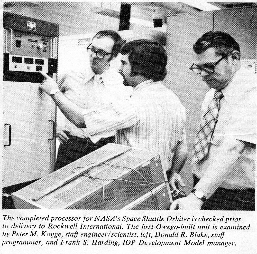
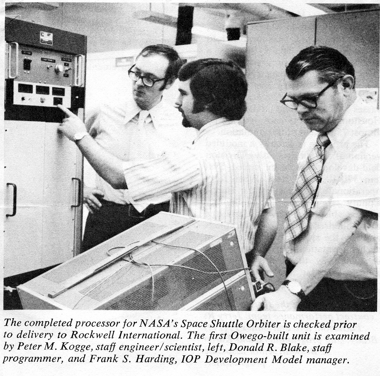
The first microcomputer: The transfluxor-powered Arma Micro Computer from 1962

What would you say is the first microcomputer?1 The Apple I from 1976? The Altair 8800 from 1974? Perhaps the lesser-known Micral N (1973) or Q1 (1972)? How about the Arma Micro Computer from way back in 1962. The Arma Micro Computer was a compact 20-pound transistorized computer, designed for applications in space such as inertial or celestial navigation, steering, radar, or engine control.

Obviously, the Arma Micro Computer is not a microcomputer according to modern definitions, since its processor was made from discrete components. But it's an interesting computer in many ways. First, it is an example of the aerospace computers of the 1960s, advanced systems that are now almost entirely forgotten. People think of 1960s computers as room-filling mainframes, but there was a whole separate world of cutting-edge miniaturized aerospace computers. (Taking up just 0.4 cubic feet, the Arma Micro Computer was smaller than an Apple II.) Second, the Arma Micro Computer used strange components such as transfluxors and had an unusual 22-bit serial architecture. Finally, the Arma Micro Computer evolved into a series of computers used on Navy ships and submarines, the E-2C Hawkeye airborne early warning plane, the Concorde, and even Air Force One.

The Arma Micro Computer

The Arma Micro Computer, with a circuit board on top. Click this image (or any other) for a larger version. Photo courtesy of Daniel Plotnick.

The Arma Micro Computer, with a circuit board on top. Click this image (or any other) for a larger version. Photo courtesy of Daniel Plotnick.

The Micro Computer used 22-bit words, which may seem like a strange size from the modern perspective. But there's no inherent need for a word size to be a power of 2. In particular, the Micro Computer was designed for mathematical calculations, not dealing with 8-bit characters. The word size was selected to provide enough accuracy for its navigational tasks.

Another strange aspect of the Micro Computer is that it was a serial machine, sequentially operating on one bit of a word at a time.2 This approach was often used in early machines because it substantially reduced the amount of hardware required: it only needs a 1-bit data bus and a 1-bit ALU. The downside is that a serial machine is much slower because each 22-bit word takes 22 clock cycles (plus 5 cycles of overhead). As a result, the Micro Computer executed just 36000 operations per second, despite its 1 megahertz clock speed.

Ad for the Arma Micro Computer (called the MICRO here). Source: Electronics, July 27, 1962.

Ad for the Arma Micro Computer (called the MICRO here). Source: Electronics, July 27, 1962.

The Micro Computer had a small instruction set of 19 instructions.3 It included multiply, divide, and square root, instructions that weren't implemented in early microprocessors. This illustrates how early microprocessors were a significant step backward in functionality. Moreover, the multiply, divide, and square root instructions used a separate arithmetic unit, so they could execute in parallel with other arithmetic instructions. Because the Micro Computer needed to interact with spacecraft systems, it had a focus on I/O, with 120 digital inputs or outputs, configured as needed for a particular mission.

Circuits

The Micro Computer was built from silicon transistors and diodes, using diode-transistor logic. The construction technique was somewhat unusual. The basic circuits were the flip-flop, the complementary buffer (i.e. an inverter), and the diode gate. Each basic circuit was constructed on a small wafer, .77 inches on a side.5 The photo below shows wafers for a two-transistor flip-flop and two diode gates. Each wafer had up to 16 connection tabs on the edges. These wafers are analogous to integrated circuits, but constructed from discrete components.

Three circuit modules from the Arma Micro Computer. Image from "The Arma Micro Computer for Space Applications".

Three circuit modules from the Arma Micro Computer. Image from "The Arma Micro Computer for Space Applications".

The wafers were mounted on printed circuit boards, with up to 22 wafers on a board. Pairs of boards were mounted back to back with polyurethane foam between the boards to form a "sandwich", which was conformally coated. The result was a module that was protected against the harsh environment of a missile or spacecraft. The computer could handle a shock of 100 g's and temperatures of 0°C to 85°C as well as 100% humidity or a vacuum.

Because the Micro Computer was a serial machine, its bits were constantly moving. For register storage such as the accumulator, it used six magnetostrictive torsional delay lines, storing a sequence of bits as physical twists that formed pulses racing through a long coil of wire.

The photo below shows the Arma Micro Computer with the case removed. If you look closely, you can see the 22 small circuit wafers mounted on each printed circuit board. The memory driver boards and delay lines are towards the back, spaced more widely than the other printed circuit boards. The cable harness underneath the boards provides the connections between boards.4

Circuit boards inside the Arma Micro Computer. Photo courtesy of Daniel Plotnick.

Circuit boards inside the Arma Micro Computer. Photo courtesy of Daniel Plotnick.

Transfluxors

One of the most unusual parts of the Micro Computer was its storage. Computers at the time typically used magnetic core memory, with each bit stored in a tiny ferrite ring, magnetized either clockwise or counterclockwise to store a 0 or 1. One drawback of standard core memory was that the process of reading a core also cleared the core, requiring data to be written back after a read.

Diagram of Arma's memory system. From patent 3048828.

Diagram of Arma's memory system. From patent 3048828.

The Micro Computer used ferrite cores, but these were "two-aperture" cores, with a larger hole and a smaller hole, as shown above. Data is written to the "major aperture" and read from the "minor aperture". Although the minor aperture switches state and is erased during a read, the major aperture retains the bit, allowing the minor aperture to be switched back to its original state. Thus, unlike regular core memory, transfluxors don't lose their data when reading.

The resulting system is called non-destructive readout (NDRO), compared to the destructive readout (DRO) of regular core memory.6 The Micro Computer used non-destructive readout memory to ensure that the program memory remained uncorrupted. In contrast, if a program is stored in regular core memory, each instruction must be written back as it is executed, creating the possibility that a transient could corrupt the software. By using transfluxors, this possibility of error is eliminated. (In either case, core memory has the convenient property that data is preserved when power is removed, since data is stored magnetically. With modern semiconductor memory, you lose data when the power goes off.)

The photo below shows a compact transfluxor-based storage module used in the Micro Computer, holding 512 words. In total, the computer could hold up to 7808 words of program memory and 256 words of data memory. It appears that transfluxors didn't live up to their promise, since most computers used regular core memory until semiconductor memory took over in the early 1970s.

Transfluxor-based core memory module from the Arma Micro Computer. Image from "The Arma Micro Computer for Space Applications".

Transfluxor-based core memory module from the Arma Micro Computer. Image from "The Arma Micro Computer for Space Applications".

Arma's history and the path to the Micro Computer

The Arma Engineering Company was founded in 1918 and built advanced military equipment.7 Its first product was a searchlight for the Navy, followed by a gyroscopic compass and analog computers for naval gun targeting. In 1939, Arma produced the Torpedo Data Computer, a remarkable electromechanical analog computer. US submarines used this computer to track target ships and automatically aim torpedos. The Torpedo Data Computer performed complex trigonometric calculations and integration to account for the motion of the target ship and the submarine. While the Torpedo Data Computer performed well, the Navy's Mark 14 torpedo had many problems—running too deep, exploding too soon, or failing to explode—making torpedoes often ineffectual even with a perfect hit.

The Torpedo Data Computer Mark III in the USS Pampanito.

The Torpedo Data Computer Mark III in the USS Pampanito.

Arma underwent major corporate changes due to World War II. Before the war, the German-owned Bosch Company built vehicle starters and aircraft magnetos in the United States. When the US entered World War II in 1941, the government was concerned that a German-controlled company was manufacturing key military hardware so the Office of Alien Property Custodian took over the Bosch plant. In 1948, the banking group that controlled Arma bought Bosch from the Office of the Alien Property Custodian, merging them into the American Bosch Arma Corporation (AMBAC).8 (Arma had earlier received the rights to gyrocompass technology from the German Anschutz company, seized by the Navy after World War I, so Arma benefitted twice from wartime government seizures.)

In the mid-1950s, Arma moved into digital computers, building an inertial guidance computer for the Atlas nuclear missile program. America's first ICBM was the Atlas missile, which became operational in 1959. The first Atlas missiles used radio guidance from the launch site to direct the missile. Since radio signals could be jammed by the enemy, this wasn't a robust solution.

The solution to missile guidance was an inertial navigation system. By using sensitive gyroscopes and accelerometers, a missile could continuously track its position and velocity without any external input, making it unjammable. A key developer of this system was Arma's Wen Tsing Chow, one of the driving forces behind digital aviation computers. He faced extreme skepticism in the 1950s for the idea of putting a computer in a missile. One general mocked him, asking "Where are you going to put the five Harvard professors you'll need to keep it running?" But computerized navigation was successful and in 1961, the Atlas missile was updated to use the Arma inertial guidance computer. It was said to be the first production airborne digital computer.9 Wen Tsing Chow also invented the programmable read-only memory (PROM), allowing missile targeting information to be programmed into a computer outside the factory.

Wen Tsing Chow, computer engineer, with Arma Micro Computer. From Control Engineering, January 1963, page 19. Courtesy of Daniel Plotnick.

Wen Tsing Chow, computer engineer, with Arma Micro Computer. From Control Engineering, January 1963, page 19. Courtesy of Daniel Plotnick.

The photo below shows the Atlas ICBM's guidance system. The Arma W-107A computer is at the top and the gyroscopes are in the middle. This computer was an 18-bit serial machine running at 143.36 kHz. It ran a hard-wired program that integrated the accelerometer information and solved equations for the crossrange error function, range error function, and gravity, making these computations every half second.10 The computer weighed 240 pounds and consumed 1000 watts. The computer contained about 36,000 components: discrete transistors, diodes, resistors, and capacitors mounted on 9.5" × 6.5" printed-circuit boards. On the ground, the computer was air-cooled to 55 °F, but there was no cooling after launch as the computer only operated for five minutes of powered flight and wouldn't overheat during that time.

Guidance system for Atlas ICBM.  From "Atlas Inertial Guidance System" by John Heiderstadt. Photo unclassified in 1967.

Guidance system for Atlas ICBM. From "Atlas Inertial Guidance System" by John Heiderstadt. Photo unclassified in 1967.

The Atlas wasn't originally designed for a computerized guidance system so there wasn't room inside the missile for the computer. To get around this, a large pod was stuck on the side of the missile to hold the computer and gyroscopes, as indicated in the photo below. This doesn't look aerodynamic, but I guess it worked.

Atlas missile. Arrow indicates the pod containing the Arma guidance computer and inertial navigation system. Original photo by Robert DuHamel, CC BY-SA 3.0.

Atlas missile. Arrow indicates the pod containing the Arma guidance computer and inertial navigation system. Original photo by Robert DuHamel, CC BY-SA 3.0.

The Atlas guidance computer (left, below) consisted of three aluminum sections called "decks". The top deck held two replaceable target constant units, each providing 54 navigation constants that specified a target. The constants were stored in a stack of printed circuit boards 16" × 8" × 1.5", covered in over a thousand diodes, Wen Tsing Chow's PROM memory. A target was programmed into the stack by a rack of equipment that would selectively burn out diodes, changing the corresponding bit to a 1. (This is why programming a PROM is referred to as "burning the PROM".11) The diode matrix was later replaced with a transfluxor memory array, which had the advantage that it could be reprogrammed as necessary. The top deck also had connectors for the accelerometer inputs, the outputs, and connections for ground support equipment. The bottom deck had power connectors for 28 volts DC and 115V 400 Hz 3-phase AC. In the bottom deck, quartz delay lines were used for storage, representing bits as acoustic waves. Twelve circuit cards, each with a faceted quartz block four inches in diameter, provided a total of 32 words of storage.

Three generations of Arma Computers: the W-107A Atlas ICBM guidance computer,  the Lightweight Airborne Digital Computer, and the Arma Micro Computer (perhaps a prototype). Photo courtesy of Daniel Plotnick.

Three generations of Arma Computers: the W-107A Atlas ICBM guidance computer, the Lightweight Airborne Digital Computer, and the Arma Micro Computer (perhaps a prototype). Photo courtesy of Daniel Plotnick.

Arma considered the Micro Computer the third generation of its airborne computers. The first generation was the Atlas guidance computer, constructed from germanium transistors and diodes (in the pre-silicon era). The second-generation computer moved to silicon transistors and diodes. The third-generation computers still used discrete components, but mounted on the small square wafers. The third generation also had a general-purpose architecture and programmable transfluxor memory instead of a hard-wired program.

After the Micro Computer

Arma continued to develop computers, improving the Arma Micro Computer. The Micro C computer (1965) was developed for Navy ships and submarines. Much like the original Micro, the Micro C used transfluxor storage, but increased the clock frequency to 972 kHz. The computer was much larger: 3.87 cubic feet and 150 pounds. This description states that "the machine is an outgrowth of the ARMA product line of micro computers and is logically and electrically similar to micro-computers designed for missile environments."

Module from the Arma Micro-C Computer. Photo courtesy of Daniel Plotnick.

Module from the Arma Micro-C Computer. Photo courtesy of Daniel Plotnick.

In mid-1966, Arma introduced the Micro D computer, built from TTL integrated circuits. Like the original Micro, this computer was serial, but the Micro D had a word length of 18 bits and ran at 1.5 MHz. It weighed 5.25 pounds and was very compact, just 0.09 ft3. Instead of transfluxors, the Micro D used regular magnetic core memory, 4K to 31K words.

The Arma Micro-D 1801 computer. The 1808 was a slightly larger model. Photo courtesy of Daniel Plotnick.

The Arma Micro-D 1801 computer. The 1808 was a slightly larger model. Photo courtesy of Daniel Plotnick.

The widely-used Litton LTN-51 inertial navigation system was built around the Arma Micro-D computer.12 This navigation system was designed for commercial aircraft, but was also used for military applications, ships, and NASA aircraft. Aircraft from early Concordes to Air Force One used the LTN-51 for navigation. The photo below shows a navigation unit with the Arma Micro-D computer in the lower left and the gyroscope unit on the right.

Litton LTN-51 inertial navigation system.  Photo courtesy of pascal mz, concordescopia.com.

Litton LTN-51 inertial navigation system. Photo courtesy of pascal mz, concordescopia.com.

In early 1968, the Arma Portable Micro D was introduced, a 14-pound battery-powered computer also called the Celestial Data Processor. This handheld computer was designed for navigation in crewed earth orbital flight, determining orbital parameters from stadimeter and sextant measurements performed by astronauts. As far as I can tell, this computer never made it beyond the prototype stage.

The Arma Celestial Data Processor (source).

The Arma Celestial Data Processor (source).

Conclusions

The Arma Micro Computer is just one of the dozens of compact aerospace computers of the 1960s, a category that is mostly forgotten and ignored. Another example is the Delco MAGIC I (1961), said to be the "first complete airborne computer to have its logic functions mechanized exclusively with integrated circuits". IBM's 4 Pi series started in 1966 and was used in many systems from the F-15 to the Space Shuttle. By 1968, denser MOS/LSI chips were used in general-purpose aerospace computers such as the Rockwell MOS GP and the Texas Instruments Model 2502 LSI Computer. 13

Arma also illustrates that a company can be on the cutting edge of technology for decades and then suddenly go out of business and be forgotten. After some struggles, Arma was acquired by United Technologies in 1978 for $210 million and was then shut down in 1982. (The German Bosch corporation remains, now a large multinational known for products such as dishwashers, auto parts, and power tools.) Looking at a list of aerospace computers shows many innovative but vanished companies: Univac, Burroughs, Sperry (now all Unisys), AC Electronics (now part of Raytheon), Autonetics (acquired by Boeing), RCA (bought by GE), and TRW (acquired by Northrop Grumman).

Finally, the Micro Computer illustrates that terms such as "microcomputer" are not objective categories but are social constructs. At first, it seems obvious that the Arma Micro Computer is not a real microcomputer. If you consider a microcomputer to be a computer built around a microprocessor, that's true. (Although "microprocessor" is also not as clear as you might think.) But a microcomputer can also be defined as "A small computer that includes one or more input/output units and sufficient memory to execute instructions" (according to the IBM Dictionary of Computing, 1994)14 and the Arma Micro Computer meets that definition. The "microcomputer" is a shifting concept, changing from the 1960s to the 1990s to today.

For more, follow me on Twitter @kenshirriff or RSS for updates. I'm also on Mastodon as @[email protected]. Thanks to Daniel Plotnick for providing a great deal of information and photos. Thanks to John Hartman for obtaining an obscure conference proceedings for me.

Notes and references

  1. I should mention the danger of "firsts" from a historical perspective. Historian Michael Williams advised "not to use the word 'first'" and said, "If you add enough adjectives to a description you can always claim your own favorite." (See ENIAC in Action, p7.)

    The first usage of "micro-computer" that I could find is from 1956. In Isaac Asimov's short story "The Dying Night", he mentions a "micro-computer" in passing: "In recent years, it [the handheld scanner] had become the hallmark of the scientist, much as the stethoscope was that of the physician and the micro-computer that of the statistician."

    Another interesting example of a "micro-computer" is the Texas Instruments Semiconductor Network Computer. This palm-sized computer is often considered the first integrated-circuit computer. It was an 11-bit serial computer running at 100 kHz, built out of RS flip-flops, NOR gates, and logic drivers. The 1961 article below described this computer as a "micro-computer", although this was a one-off use of the term, not the computer's name. This brochure describes the Semiconductor Network Computer in more detail and Semiconductor Networks are described in detail in this article. Unlike modern ICs, these integrated circuits used flying wires for internal connections rather than a deposited metal layer, making their design a dead end.

    The Texas Instruments Semiconductor Network Computer. From Computers and Automation, Dec. 1961.

    The Texas Instruments Semiconductor Network Computer. From Computers and Automation, Dec. 1961.


  2. Most of the information on the Arma Micro Computer in this article is from "The Arma Micro Computer for Space Applications", by E. Keonjian and J. Marx, Spaceborne Computing Engineering Conference, 1962, pages 103-116. 

  3. The Arma Micro Computer's instruction set consisted of 19 22-bit instructions, shown below.

    Instruction set of the Arma Micro Computer. Figure from "The Arma Micro Computer for Space Applications".

    Instruction set of the Arma Micro Computer. Figure from "The Arma Micro Computer for Space Applications".


  4. This block diagram shows the structure of the Micro Computer. The accumulator register (AC) is used for all data transfers as well as addition and subtraction. The multiply-divide register is used for multiplication, division, and square roots. The product register (PR), quotient register (QR), and square root register (SR) are used by the corresponding instructions. The data buffer register (S) holds data moving in or out of storage; it is shown with two 11-bit parts.

    Block diagram of the Arma Micro Computer. Figure from "The Arma Micro Computer for Space Applications".

    Block diagram of the Arma Micro Computer. Figure from "The Arma Micro Computer for Space Applications".

    For control logic, the location counter (L) is the 13-bit program counter. For a subroutine call, the current address can be stored in the recall register (RR), which acts as a link register to hold the return address. (The RR is not shown on the diagram because it is held in memory.) Instruction decoding uses the instruction register (I), with the next instruction in the instruction buffer (B). The operand register (P) contains the 13-bit address from an instruction, while the remaining register (R) is used for I/O addressing. 

  5. Arma's original plan was to mount circuits on ceramic wafers. Resistors would be printed onto the wafer and wiring silk-screened. (This is similar to IBM's SLT modules (1964), although IBM mounted diode and transistors as bare dies rather than components.) However, the Micro Computer ended up using epoxy-glass wafers with small, but discrete components: standard TO-46 transistors, "fly-speck" diodes, and 1/10 watt resistors. I don't see much advantage to these wafers over mounting the components directly on the printed-circuit board; maybe standardization is the benefit. 

  6. The Micro Computer used an unusual mechanism to select a word to read or write. Most computers used a grid of selection wires; by energizing an X and a Y wire at the same time, the corresponding core was selected. The key idea of this "coincident-current" approach is that each wire has half the current necessary to flip a core, so the core with the energized X and Y wires will have enough current to flip. This puts tight constraints on the current level, since too much current will flip all the cores along the wire, but not enough current will not flip the selected core. What makes this difficult is that the properties of a core change with temperature, so either the cores need to be temperature-stabilized or the current needs to be adjusted based on the temperature.

    The Micro Computer instead used a separate wire for each word, so as long as the current is large enough, the cores will flip. This approach avoids the issues with temperature sensitivity, an important concern for a computer that needs to handle the large temperature swings of a spacecraft, not an air-conditioned data center. Unfortunately, it requires much more wiring. Specifically, the large advantage of the coincident-current approach is that an N×N grid of wires lets you select N2 words. With the Micro Computer approach, N wires only select N words, so the scalability is much worse.

    For more on Arma's memory systems, see patents: Memory Device, 3048828 and Multiaperture Core Memory Matrix, 3289181

  7. The capitalization of Arma vs. ARMA is inconsistent. It often appears in all-caps, but both forms are used, sometimes in the same article. "Arma" is not an acronym; the name came from the names of its founders: Arthur Davis and David Mahood (source: Between Human and Machine, p54). I suspect a 1960s corporate branding effort was responsible for the use of all-caps. 

  8. For more on the corporate history of Arma, see IRE Pulse, March 1958, p9-10. Details of corporate politics and what went wrong are here. More information on the financial ups and downs of Arma is in "Charles Perelle's Spacemanship", Fortune, January 1959, an article that focused on Charles Perelle, the president of American Bosch Arma. 

  9. Wikipedia says that Arma's guidance computer was "the first production airborne digital computer". However, the Hughes Digitair (1958) has also been called "the first airborne digital computer in actual production." Another source says the Arma computer was the "first all-solid-state, high-reliability, space-borne digital computer." The TRADIC (Transistorized Airborne Digital Computer) (1954) was earlier, but was a prototype system, not a production system. In turn, the TRADIC is said by some to be the first fully transistorized computer, but that depends on exactly how you interpret "fully".

    This is another example of how the "first" depends on the specific adjectives used. 

  10. The information on the Arma W-107A computer is from "Atlas Inertial Guidance System: As I Remember It" by Principal Engineer John Heiderstadt. 

  11. Chow Wen Tsing's PROM patent discusses the term "burning", explaining that it refers to burning out the diodes electrically. To widen the patent, he clarifies that "The term 'blowing out' or 'burning out' further includes any process which, by means less drastic than actual destruction of the non-linear elements, effects a change of the circuit impedance to a level which makes the particular circuit inoperative." This description prevented someone from trying to get around the patent by stating that nothing was really burning. 

  12. Details on the LTN-51 navigation system and its uses are in this document

  13. For more information on early aerospace computers, see State-of-the-art of Aerospace Digital Computers (1967), updated as Trends in Aerospace Digital Computer Design (1969). Also see the 1970 Survey of Military CPUs. Efficient partitioning for the batch-fabricated fourth generation computer (1968) discusses how "The computer industry is on the verge of an upheaval" from new hardware including LSI and fast ROMs, and describes various LSI aerospace computers. 

  14. The "IBM Dictionary of Computing" (1994) has two definitions of "microcomputer": "(1) A digital computer whose processing unit consists of one or more microprocessors, and includes storage and input/output facilities. (2) A small computer that includes one or more input/output units and sufficient memory to execute instructions; for example a personal computer. The essential components of a microcomputer are often contained within a single enclosure." The latter definition was from an ISO/IEC draft standard for terminology so it is somewhat "official". 

Inside the mechanical Bendix Air Data Computer, part 5: motor/tachometers

The Bendix Central Air Data Computer (CADC) is an electromechanical analog computer that uses gears and cams for its mathematics. It was a key part of military planes such as the F-101 and the F-111 fighters, computing airspeed, Mach number, and other "air data". The rotating gears are powered by six small servomotors, so these motors are in a sense the fundamental component of the CADC. In the photo below, you can see one of the cylindrical motors near the center, about 1/3 of the way down.

The servomotors in the CADC are unlike standard motors. Their name—"Motor-Tachometer Generator" or "Motor and Rate Generator"1—indicates that each unit contains both a motor and a speed sensor. Because the motor and generator use two-phase signals, there are a total of eight colorful wires coming out, many more than a typical motor. Moreover, the direction of the motor can be controlled, unlike typical AC motors. I couldn't find a satisfactory explanation of how these units worked, so I bought one and disassembled it. This article (part 5 of my series on the CADC2) provides a complete teardown of the motor/generator and explain how it works.

The Bendix MG-1A Central Air Data Computer with the case removed, showing the compact gear mechanisms inside. Click this image (or any other) for a larger version.

The Bendix MG-1A Central Air Data Computer with the case removed, showing the compact gear mechanisms inside. Click this image (or any other) for a larger version.

The image below shows a closeup of two motors powering one of the pressure signal outputs. Note the bundles of colorful wires to each motor, entering in two locations. At the top, the motors drive complex gear trains. The high-speed motors are geared down by the gear trains to provide much slower rotations with sufficient torque to power the rest of the CADC's mechanisms.

Two motor/generators in the pressure section of the CADC. The one at the back is mostly hidden.

Two motor/generators in the pressure section of the CADC. The one at the back is mostly hidden.

The motor/tachometer that we disassembled is shorter than the ones in the CADC (despite having the same part number), but the principles are the same. We started by removing a small C-clip on the end of the motor and and unscrewing the end plate. The unit is pretty simple mechanically. It has bearings at each end for the rotor shaft. There are four wires for the motor and four wires for the tachometer.3

The motor disassembled to show the internal components.

The motor disassembled to show the internal components.

The rotor (below) has two parts on the shaft. the left part is for the motor and the right drum is for the tachometer. The left part is a squirrel-cage rotor4 for the motor. It consists of conducting bars (light-colored) on an iron core. The conductors are all connected at both ends by the conductive rings at either end. The metal drum on the right is used by the tachometer. Note that there are no electrical connections between the rotor components and the rest of the motor: there are no brushes or slip rings. The interaction between the rotor and the windings in the body of the motor is purely magnetic, as will be explained.

The rotor and shaft.

The rotor and shaft.

The motor/tachometer contains two cylindrical stators that create the magnetic fields, one for the motor and one for the tachometer. The photo below shows the motor stator inside the unit after removing the tachometer stator. The stators are encased in hard green plastic and tightly pressed inside the unit. In the center, eight metal poles are visible. They direct the magnetic field onto the rotor.

Inside the motor after removing the tachometer winding.

Inside the motor after removing the tachometer winding.

The photo below shows the stator for the tachometer, similar to the stator for the motor. Note the shallow notches that look like black lines in the body on the lower left. These are probably adjustments to the tachometer during manufacturing to compensate for imperfections. The adjustments ensure that the magnetic fields are nulled out so the tachometer returns zero voltage when stationary. The metal plate on top shields the tachometer from the motor's magnetic fields.

The stator for the tachometer.

The stator for the tachometer.

The poles and the metal case of the stator look solid, but they are not. Instead, they are formed from a stack of thin laminations. The reason to use laminations instead of solid metal is to reduce eddy currents in the metal. Each lamination is varnished, so it is insulated from its neighbors, preventing the flow of eddy currents.

One lamination from the stack of laminations that make up the winding. The lamination suffered some damage during disassembly; it was originally round.

One lamination from the stack of laminations that make up the winding. The lamination suffered some damage during disassembly; it was originally round.

In the photo below, I removed some of the plastic to show the wire windings underneath. The wires look like bare copper, but they have a very thin layer of varnish to insulate them. There are two sets of windings (orange and blue, or red and black) around alternating metal poles. Note that the wires run along the pole, parallel to the rotor, and then wrap around the pole at the top and bottom, forming oblong coils around each pole.5 This generates a magnetic field through each pole.

Removing the plastic reveals the motor windings.

Removing the plastic reveals the motor windings.

The motor

The motor part of the unit is a two-phase induction motor with a squirrel-cage rotor.6 There are no brushes or electrical connections to the rotor, and there are no magnets, so it isn't obvious what makes the rotor rotate. The trick is the "squirrel-cage" rotor, shown below. It consists of metal bars that are connected at the top and bottom by rings. Assume (for now) that the fixed part of the motor, the stator, creates a rotating magnetic field. The important principle is that a changing magnetic field will produce a current in a wire loop.7 As a result, each loop in the squirrel-cage rotor will have an induced current: current will flow up9 the bars facing the north magnetic field and down the south-facing bars, with the rings on the end closing the circuits.

A squirrel-cage rotor. The numbered parts are (1) shaft, (2) end cap, (3) laminations, and (4) splines to hold the laminations. Image from Robo Blazek.

A squirrel-cage rotor. The numbered parts are (1) shaft, (2) end cap, (3) laminations, and (4) splines to hold the laminations. Image from Robo Blazek.

But how does the stator produce a rotating magnetic field? And how do you control the direction of rotation? The next important principle is that current flowing through a wire produces a magnetic field.8 As a result, the currents in the squirrel cage rotor produce a magnetic field perpendicular to the cage. This magnetic field causes the rotor to turn in the same direction as the stator's magnetic field, driving the motor. Because the rotor is powered by the induced currents, the motor is called an induction motor.

The diagram below shows how the motor is wired, with a control winding and a reference winding. Both windings are powered with AC, but the control voltage either lags the reference winding by 90° or leads the reference winding by 90°, due to the capacitor. Suppose the current through the control winding lags by 90°. First, the reference voltage's sine wave will have a peak, producing the magnetic field's north pole at A. Next (90° later), the control voltage will peak, producing the north pole at B. The reference voltage will go negative, producing a south pole at A and thus a north pole at C. The control voltage will go negative, producing a south pole at B and a north pole at D. This cycle will repeat, with the magnetic field rotating counter-clockwise from A to D. Conversely, if the control voltage leads the reference voltage, the magnetic field will rotate clockwise. This causes the motor to spin in one direction or the other, with the direction controlled by the control voltage. (The motor has four poles for each winding, rather than the one shown below; this increases the torque and reduces the speed.)

Diagram showing the servomotor wiring.

Diagram showing the servomotor wiring.

The purpose of the capacitor is to provide the 90° phase shift so the reference voltage and the control voltage can be driven from the same single-phase AC supply (in this case, 26 volts, 400 hertz). Switching the polarity of the control voltage reverses the direction of the motor.

There are a few interesting things about induction motors. You might expect that the motor would spin at the same rate as the rotating magnetic field. However, this is not the case. Remember that a changing magnetic field induces the current in the squirrel-cage rotor. If the rotor is spinning at the same rate as the magnetic field, the rotor will encounter an unchanging magnetic field and there will be no current in the bars of the rotor. As a result, the rotor will not generate a magnetic field and there will be no torque to rotate it. The consequence is that the rotor must spin somewhat slower than the magnetic field. This is called "slippage" and is typically a few percent of the full speed, with more slippage as more torque is required.

Many household appliances use induction motors, but how do they generate a rotating magnetic field from a single-phase AC winding? The problem is that the magnetic field in a single AC winding will just flip back and forth, so the motor will not turn in either direction. One solution is a shaded-pole motor, which puts a copper bar around part of each pole to break the symmetry and produce a weakly rotating magnetic field. More powerful induction motors use a startup winding with a capacitor (analogous to the control winding). This winding can either be switched out of the circuit once the motor starts spinning,10 or used continuously, called a permanent-split capacitor (PSC) motor. The best solution is three-phase power (if available); a three-phase winding automatically produces a rotating magnetic field.

Tachometer/generator

The second part of the unit is the tachometer generator, sometimes called the rate unit.11 The purpose of the generator is to produce a voltage proportional to the speed of the shaft. The unusual thing about this generator is that it produces a 400-hertz output that is either in phase with the input or 180° out of phase. This is important because the phase indicates which direction the shaft is turning. Note that a "normal" generator is different: the output frequency is proportional to the speed.

The diagram below shows the principle behind the generator. It has two stator windings: the reference coil that is powered at 400 Hz, and the output coil that produces the output signal. When the rotor is stationary (A), the magnetic flux is perpendicular to the output coil, so no output voltage is produced. But when the rotor turns (B), eddy currents in the rotor distort the magnetic field. It now couples with the output coil, producing a voltage. As the rotor turns faster, the magnetic field is distorted more, increasing the coupling and thus the output voltage. If the rotor turns in the opposite direction (C), the magnetic field couples with the output coil in the opposite direction, inverting the output phase. (This diagram is more conceptual than realistic, with the coils and flux 90° from their real orientation, so don't take it too seriously. As shown earlier, the coils are perpendicular to the rotor so the real flux lines are completely different.)

Principle of the drag-cup rate generator. From Navy electricity and electronics training series: Principles of synchros, servos, and gyros, Fig 2-16

But why does the rotating drum change the magnetic field? It's easier to understand by considering a tachometer that uses a squirrel-cage rotor instead of a drum. When the rotor rotates, currents will be induced in the squirrel cage, as described earlier with the motor. These currents, in turn, generate a perpendicular magnetic field, as before. This magnetic field, perpendicular to the orginal field, will be aligned with the output coil and will be picked up. The strength of the induced field (and thus the output voltage) is proportional to the speed, while the direction of the field depends on the direction of rotation. Because the primary coil is excited at 400 hertz, the currents in the squirrel cage and the resulting magnetic field also oscillate at 400 hertz. Thus, the output is at 400 hertz, regardless of the input speed.

Using a drum instead of a squirrel cage provides higher accuracy because there are no fluctuations due to the discrete bars. The operation is essentially the same, except that the currents pass through the metal of the drum continuously instead of through individual bars. The result is eddy currents in the drum, producing the second magnetic field. The diagram below shows the eddy currents (red lines) from a metal plate moving through a magnetic field (green), producing a second magnetic field (blue arrows). For the rotating drum, the situation is similar except the metal surface is curved, so both field arrows will have a component pointing to the left. This creates the directed magnetic field that produces the output.

A diagram showing eddy currents in a metal plate moving under a magnet, Image from Chetvorno.

A diagram showing eddy currents in a metal plate moving under a magnet, Image from Chetvorno.

The servo loop

The motor/generator is called a servomotor because it is used in a servo loop, a control system that uses feedback to obtain precise positioning. In particular, the CADC uses the rotational position of shafts to represent various values. The servo loops convert the CADC's inputs (static pressure, dynamic pressure, temperature, and pressure correction) into shaft positions. The rotations of these shafts power the gears, cams, and differentials that perform the computations.

The diagram below shows a typical servo loop in the CADC. The goal is to rotate the output shaft to a position that exactly matches the input voltage. To accomplish this, the output position is converted into a feedback voltage by a potentiometer that rotates as the output shaft rotates.12 The error amplifier compares the input voltage to the feedback voltage and generates an error signal, rotating the servomotor in the appropriate direction. Once the output shaft is in the proper position, the error signal drops to zero and the motor stops. To improve the dynamic response of the servo loop, the tachometer signal is used as a negative feedback voltage. This ensures that the motor slows as the system gets closer to the right position, so the motor doesn't overshoot the position and oscillate. (This is sort of like a PID controller.)

Diagram of a servo loop in the CADC.

Diagram of a servo loop in the CADC.

The error amplifier and motor drive circuit for a pressure transducer are shown below. Because of the state of electronics at the time, it took three circuit boards to implement a single servo loop. The amplifier was implemented with germanium transistors (since silicon transistors were later). The transistors weren't powerful enough to drive the motors directly. Instead, magnetic amplifiers (the yellow transformer-like modules at the front) powered the servomotors. The large rectangular capacitors on the right provided the phase shift required for the control voltage.

One of the three-board amplifiers for the pressure transducer.

One of the three-board amplifiers for the pressure transducer.

Conclusions

The Bendix CADC used a variety of electromechanical devices including synchros, control transformers, servo motors, and tachometer generators. These were expensive military-grade components driven by complex electronics. Nowadays, you can get a PWM servo motor for a few dollars with the gearing, feedback, and control circuitry inside the motor housing. These motors are widely used for hobbyist robotics, drones, and other applications. It's amazing that servo motors have gone from specialized avionics hardware to an easy-to-use, inexpensive commodity.

A modern DC servo motor. Photo by Adafruit (CC BY-NC-SA 2.0 DEED).

A modern DC servo motor. Photo by Adafruit (CC BY-NC-SA 2.0 DEED).

Follow me on Twitter @kenshirriff or RSS for updates. I'm also on Mastodon as @oldbytes.space@kenshirriff. Thanks to Joe for providing the CADC. Thanks to Marc Verdiell for disassembling the motor.

Notes and references

  1. The two types of motors in the CADC are part number "FV-101-19-A1" and part number "FV-101-5-A1" (or FV101-5A1). They are called either a "Tachometer Rate Generator" or "Tachometer Motor Generator", with both names applied to the same part number. The "19" and "5" units look the same, with the "19" used for one pressure servo loop and the "5" used everywhere else.

    The motor that I got is similar to the ones in the CADC, but shorter. The difference in size is mysterious since both have the Bendix part number FV-101-5-A1.

    For reference, the motor I disassembled is labeled:

    Cedar Division Control Data Corp. ST10162 Motor Tachometer F0: 26V C0: 26V TACH: 18V 400 CPS DSA-400-70C-4651 FSN6105-581-5331 US BENDIX FV-101-5-A1

    I wondered why the motor listed both Control Data and Bendix. In 1952, the Cedar Engineering Company was spun off from the Minneapolis Honeywell Regulator Company (better known as Honeywell, the name it took in 1964). Cedar Engineering produced motors, servos, and aircraft actuators. In 1957, Control Data bought Cedar Engineering, which became the Cedar Division of CDC. Then, Control Data acquired Bendix's computer division in 1963. Thus, three companies were involved. 

  2. My previous articles on the CADC are:


  3. From testing the motor, here is how I believe it is wired:
    Motor reference (power): red and black
    Motor control: blue and orange
    Generator reference (power): green and brown
    Generator out: white and yellow 

  4. The bars on the squirrel-cage rotor are at a slight angle. Parallel bars would go in and out of alignment with the stator, causing fluctuations in the force, while the angled bars avoid this problem. 

  5. This cross-section through the stator shows the windings. On the left, each winding is separated into the parts on either side of the pole. On the right, you can see how the wires loop over from one side of the pole to the other. Note the small circles in the 12 o'clock and 9 o'clock positions: cross sections of the input wires. The individual horizontal wires near the circumference connect alternating windings.

    A cross-section of the stator, formed by sanding down the plastic on the end.

    A cross-section of the stator, formed by sanding down the plastic on the end.


  6. It's hard to find explanations of AC servomotors since they are an old technology. One discussion is in Electromechanical components for servomechanisms (1961). This book points out some interesting things about a servomotor. The stall torque is proportional to the control voltage. Servomotors are generally high-speed, but low-torque devices, heavily geared down. Because of their high speed and their need to change direction, rotational inertia is a problem. Thus, servomotors typically have a long, narrow rotor compared with typical motors. (You can see in the teardown photo that the rotor is long and narrow.) Servomotors are typically designed with many poles (to reduce speed) and smaller air gaps to increase inductance. These small airgaps (e.g. 0.001") require careful manufacturing tolerance, making servomotors a precision part. 

  7. The principle is Faraday's law of induction: "The electromotive force around a closed path is equal to the negative of the time rate of change of the magnetic flux enclosed by the path." 

  8. Ampère's law states that "the integral of the magnetizing field H around any closed loop is equal to the sum of the current flowing through the loop." 

  9. The direction of the current flow (up or down) depends on the direction of rotation. I'm not going to worry about the specific direction of current flow, magnetic flux, and so forth in this article. 

  10. Once an induction motor is spinning, it can be powered from a single AC phase since the stator is rotating with respect to the magnetic field. This works for the servomotor too. I noticed that once the motor is spinning, it can operate without the control voltage. This isn't the normal way of using the motor, though. 

  11. A long discussion of tachometers is in the book Electromechanical Components for Servomechanisms (1961). The AC induction-generator tachometer is described starting on page 193.

    For a mathematical analysis of the tachometer generator, see Servomechanisms, Section 2, Measurement and Signal Converters, MCP 706-137, U.S. Army. This source also discusses sources of errors in detail. Inexpensive tachometer generators may have an error of 1-2%, while precision devices can have an error of about 0.1%. Accuracy is worse for small airborne generators, though. Since the Bendix CADC uses the tachometer output for damping, not as a signal output, accuracy is less important. 

  12. Different inputs in the CADC use different feedback mechanisms. The temperature servo uses a potentiometer for feedback. The angle of attack correction uses a synchro control transformer, which generates a voltage based on the angle error. The pressure transducers contain inductive pickups that generate a voltage based on the pressure error. For more details, see my article on the CADC's pressure transducer servo circuits

Reverse-engineering an analog Bendix air data computer: part 4, the Mach section

In the 1950s, many fighter planes used the Bendix Central Air Data Computer (CADC) to compute airspeed, Mach number, and other "air data". The CADC is an analog computer, using tiny gears and specially-machined cams for its mathematics. In this article, part 4 of my series,1 I reverse engineer the Mach section of the CADC and explain its calculations. (In the photo below, the Mach section is the middle section of the CADC.)

The Bendix MG-1A Central Air Data Computer with the case removed, showing the compact gear mechanisms inside. Click this image (or any other) for a larger version.

The Bendix MG-1A Central Air Data Computer with the case removed, showing the compact gear mechanisms inside. Click this image (or any other) for a larger version.

Aircraft have determined airspeed from air pressure for over a century. A port in the side of the plane provides the static air pressure,2 the air pressure outside the aircraft. A pitot tube points forward and receives the "total" air pressure, a higher pressure due to the air forced into the tube by the speed of the airplane. The airspeed can be determined from the ratio of these two pressures, while the altitude can be determined from the static pressure.

But as you approach the speed of sound, the fluid dynamics of air change and the calculations become very complicated. With the development of supersonic fighter planes in the 1950s, simple mechanical instruments were no longer sufficient. Instead, an analog computer calculated the "air data" (airspeed, air density, Mach number, and so forth) from the pressure measurements. This computer then transmitted the air data electrically to the systems that needed it: instruments, weapons targeting, engine control, and so forth. Since the computer was centralized, the system was called a Central Air Data Computer or CADC, manufactured by Bendix and other companies.

A closeup of the numerous gears inside the CADC. Three differential gear mechanisms are visible.

A closeup of the numerous gears inside the CADC. Three differential gear mechanisms are visible.

Each value in the Bendix CADC is indicated by the rotational position of a shaft. Compact electric motors rotate the shafts, controlled by the pressure inputs. Gears, cams, and differentials perform computations, with the results indicated by more rotations. Devices called synchros converted the rotations to electrical outputs that are connected to other aircraft systems. The CADC is said to contain 46 synchros, 511 gears, 820 ball bearings, and a total of 2,781 major parts (but I haven't counted). These components are crammed into a compact cylinder: just 15 inches long and weighing 28.7 pounds.

The equations computed by the CADC are impressively complicated. For instance, one equation is:

\[~~~\frac{P_t}{P_s} = \frac{166.9215M^7}{( 7M^2-1)^{2.5}}\]

It seems incredible that these functions could be computed mechanically, but three techniques make this possible. The fundamental mechanism is the differential gear, which adds or subtracts values. Second, logarithms are used extensively, so multiplications and divisions are implemented by additions and subtractions performed by a differential, while square roots are calculated by gearing down by a factor of 2. Finally, specially-shaped cams implement functions: logarithm, exponential, and application-specific functions. By combining these mechanisms, complicated functions can be computed mechanically, as I will explain below.

The differential

The differential gear assembly is the mathematical component of the CADC, as it performs addition or subtraction.3 The differential takes two input rotations and produces an output rotation that is the sum or difference of these rotations.4 Since most values in the CADC are expressed logarithmically, the differential computes multiplication and division when it adds or subtracts its inputs.

A closeup of a differential mechanism.

A closeup of a differential mechanism.

While the differential functions like the differential in a car, it is constructed differently, with a spur-gear design. This compact arrangement of gears is about 1 cm thick and 3 cm in diameter. The differential is mounted on a shaft along with three co-axial gears: two gears provide the inputs to the differential and the third provides the output. In the photo, the gears above and below the differential are the input gears. The entire differential body rotates with the sum, connected to the output gear at the top through a concentric shaft. (In practice, any of the three gears can be used as the output.) The two thick gears inside the differential body are part of the mechanism.

The cams

The CADC uses cams to implement various functions. Most importantly, cams compute logarithms and exponentials. Cams also implement complicated functions of one variable such as ${M}/{\sqrt{1 + .2 M^2}}$. The function is encoded into the cam's shape during manufacturing, so a hard-to-compute nonlinear function isn't a problem for the CADC. The photo below shows a cam with the follower arm in front. As the cam rotates, the follower moves in and out according to the cam's radius.

A cam inside the CADC implements a function.

A cam inside the CADC implements a function.

However, the shape of the cam doesn't provide the function directly, as you might expect. The main problem with the straightforward approach is the discontinuity when the cam wraps around. For example, if the cam implemented an exponential directly, its radius would spiral exponentially and there would be a jump back to the starting value when it wraps around. Instead, the CADC uses a clever patented method: the cam encodes the difference between the desired function and a straight line. For example, an exponential curve is shown below (blue), with a line (red) between the endpoints. The height of the gray segment, the difference, specifies the radius of the cam (added to the cam's fixed minimum radius). The point is that this difference goes to 0 at the extremes, so the cam will no longer have a discontinuity when it wraps around. Moreover, this technique significantly reduces the size of the value (i.e. the height of the gray region is smaller than the height of the blue line), increasing the cam's accuracy.5

An exponential curve (blue), linear curve (red), and the difference (gray).

An exponential curve (blue), linear curve (red), and the difference (gray).

To make this work, the cam position must be added to the linear value to yield the result. This is implemented by combining each cam with a differential gear; watch for the paired cams and differentials below. As the diagram below shows, the input (23) drives the cam (30) and the differential (25, 37-41). The follower (32) tracks the cam and provides a second input (35) to the differential. The sum from the differential produces the desired function (26).

This diagram, from Patent 2969910, shows how the cam and follower are connected to a differential.

This diagram, from Patent 2969910, shows how the cam and follower are connected to a differential.

The synchro outputs

A synchro is an interesting device that can transmit a rotational position electrically over three wires. In appearance, a synchro is similar to an electric motor, but its internal construction is different, as shown below. Before digital systems, synchros were very popular for transmitting signals electrically through an aircraft. For instance, a synchro could transmit an altitude reading to a cockpit display or a targeting system. Two synchros at different locations have their stator windings connected together, while the rotor windings are driven with AC. Rotating the shaft of one synchro causes the other to rotate to the same position.6

Cross-section diagram of a synchro showing the rotor and stators.

Cross-section diagram of a synchro showing the rotor and stators.

For the CADC, most of the outputs are synchro signals, using compact synchros that are about 3 cm in length. For improved resolution, many of the CADC outputs use two synchros: a coarse synchro and a fine synchro. The two synchros are typically geared in an 11:1 ratio, so the fine synchro rotates 11 times as fast as the coarse synchro. Over the output range, the coarse synchro may turn 180°, providing the approximate output unambiguously, while the fine synchro spins multiple times to provide more accuracy.

Examining the Mach section of the CADC

Another view of the CADC.

Another view of the CADC.

The Bendix CADC is constructed from modular sections. In this blog post, I'm focusing on the middle section, called the "Mach section" and indicated by the arrow above. This section computes log static pressure, impact pressure, pressure ratio, and Mach number and provides these outputs electrically as synchro signals. It also provides the log pressure ratio and log static pressure to the rest of the CADC as shaft rotations. The left section of the CADC computes values related to airspeed, air density, and temperature.7 The right section has the pressure sensors (the black domes), along with the servo mechanisms that control them.

I had feared that any attempt at disassembly would result in tiny gears flying in every direction, but the CADC was designed to be taken apart for maintenance. Thus, I could remove the left section of the CADC for analysis. Unfortunately, we lost the gear alignment between the sections and don't have the calibration instructions, so the CADC no longer produces accurate results.

The diagram below shows the internal components of the Mach section after disassembly. The synchros are in pairs to generate coarse and fine outputs; the coarse synchros can be distinguished because they have spiral anti-backlash springs installed. These springs prevent wobble in the synchro and gear train as the gears change direction. The gears and differentials are not visible from this angle as they are underneath the metal plate. The Pressure Error Correction (PEC) subsystem has a motor to drive the shaft and a control transformer for feedback. The Mach section has two D-sub connectors. The one on the right links the Mach section and pressure section to the front section of the CADC. The Position Error Correction (PEC) servo amplifier board plugs into the left connector. The static pressure and total pressure input lines have fittings so the lines can be disconnected from the lines from the front of the CADC.8

The Mach section with components labeled.

The Mach section with components labeled.

The photo below shows the left section of the CADC. This section meshes with the Mach section shown above. The two sections have parts at various heights, so they join in a complicated way. Two gears receive the pressure signals \( log ~ P_t / P_s \) and \( log ~ P_s \) from the Mach section. The third gear sends the log total temperature to the rest of the CADC. The electrical connector (a standard 37-pin D-sub) supplies 120 V 400 Hz power to the Mach section and pressure transducers and passes synchro signals to the output connectors.

The left part of the CADC that meshes with the Mach section.

The left part of the CADC that meshes with the Mach section.

The position error correction servo loop

The CADC receives two pressure inputs and two pressure transducers convert the pressures into rotational positions, providing the indicated static pressure \( P_{si} \) and the total pressure \( P_t \) as shaft rotations to the rest of the CADC. (I explained the pressure transducers in detail in the previous article.)

There's one complication though. The static pressure \( P_s \) is the atmospheric pressure outside the aircraft. The problem is that the static pressure measurement is perturbed by the airflow around the aircraft, so the measured pressure (called the indicated static pressure \( P_{si} \)) doesn't match the real pressure. This is bad because a "static-pressure error manifests itself as errors in indicated airspeed, altitude, and Mach number to the pilot."9

The solution is a correction factor called the Position Error Correction. This factor gives the ratio between the real pressure \( P_s \) and the measured pressure \( P_{si} \). By applying this correction factor to the indicated (i.e. measured) pressure, the true pressure can be obtained. Since this correction factor depends on the shape of the aircraft, it is generated outside the CADC by a separate cylindrical unit called the Compensator, customized to the aircraft type. The position error computation depends on two parameters: the Mach number provided by the CADC and the angle of attack provided by an aircraft sensor. The compensator determines the correction factor by using a three-dimensional cam. The vintage photo below shows the components inside the compensator.

"Static Pressure and Angle of Attack Compensator Type X1254115-1 (Cover Removed)" from Air Data Computer Mechanization.

"Static Pressure and Angle of Attack Compensator Type X1254115-1 (Cover Removed)" from Air Data Computer Mechanization.

The correction factor is transmitted from the compensator to the CADC as a synchro signal over three wires. To use this value, the CADC must convert the synchro signal to a shaft rotation. The CADC uses a motorized servo loop that rotates the shaft until the shaft position matches the angle specified by the synchro input.

The servo loop ensures that the shaft position matches the input angle.

The servo loop ensures that the shaft position matches the input angle.

The key to the servo loop is a control transformer. This device looks like a synchro and has five wires like a synchro, but its function is different. Like the synchro motor, the control transformer has three stator wires that provide the angle input. Unlike the synchro, the control transformer also uses the shaft position as an input, while the rotor winding generates an output voltage indicating the error. This output voltage indicates the error between the control transformer's shaft position and the three-wire angle input. The control transformer provides its error signal as a 400 Hz sine wave, with a larger signal indicating more error.10

The amplifier board (below) drives the motor in the appropriate direction to cancel out the error. The power transformer in the upper left is the largest component, powering the amplifier board from the CADC's 115-volt, 400 Hertz aviation power. Below it are two transformer-like components; these are the magnetic amplifiers. The relay in the lower-right corner switches the amplifier into test mode. The rest of the circuitry consists of transistors, resistors, capacitors, and diodes. The construction is completely different from modern printed circuit boards. Instead, the amplifier uses point-to-point wiring between plastic-insulated metal pegs. Both sides of the board have components, with connections between the sides through the metal pegs.

The amplifier board for the position error correction.

The amplifier board for the position error correction.

The amplifier board is implemented with a transistor amplifier driving two magnetic amplifiers, which control the motor.11 (Magnetic amplifiers are an old technology that can amplify AC signals, allowing the relatively weak transistor output to control a larger AC output.12) The motor is a "Motor / Tachometer Generator" unit that also generates a voltage based on the motor's speed. This speed signal provides negative feedback, limiting the motor speed as the error becomes smaller and ensuring that the feedback loop doesn't overshoot. The photo below shows how the amplifier board is mounted in the middle of the CADC, behind the static pressure tubing.

Side view of the CADC.

Side view of the CADC.

The equations

Although the CADC looks like an inscrutable conglomeration of tiny gears, it is possible to trace out the gearing and see exactly how it computes the air data functions. With considerable effort, I have reverse-engineered the mechanisms to create the diagram below, showing how each computation is broken down into mechanical steps. Each line indicates a particular value, specified by a shaft rotation. The ⊕ symbol indicates a differential gear, adding or subtracting its inputs to produce another value. The cam symbol indicates a cam coupled to a differential gear. Each cam computes either a specific function or an exponential, providing the value as a rotation. At the right, the outputs are either shaft rotations to the rest of the CADC or synchro outputs.

This diagram shows how the values are computed. The differential numbers are my own arbitrary numbers. Click for a larger version.

This diagram shows how the values are computed. The differential numbers are my own arbitrary numbers. Click for a larger version.

I'll go through each calculation briefly.

log static pressure

The static pressure is calculated by dividing the indicated static pressure by the pressure error correction factor. Since these values are all represented logarithmically, the division turns into a subtraction, performed by a differential gear. The output goes to two synchros, geared to provide coarse and fine outputs.13

\[log ~ P_s = log ~ P_{si} - log ~ P_{si} / P_s \]

Impact pressure

The impact pressure is the pressure due to the aircraft's speed, the difference between the total pressure and the static pressure. To compute the impact pressure, the log pressure values are first converted to linear values by exponentiation, performed by cams. The linear pressure values are then subtracted by a differential gear. Finally, the impact pressure is output through two synchros, coarse and fine in an 11:1 ratio.

\[ P_t - P_s = exp(log ~ P_t) - exp(log ~ P_s) \]

log pressure ratio

The log pressure ratio \( P_t/P_s \) is the ratio of total pressure to static pressure. This value is important because it is used to compute the Mach number, true airspeed, and log free air temperature. The Mach number is computed in the Mach section as described below. The true airspeed and log free air temperature are computed in the left section. The left section receives the log pressure ratio as a rotation. Since the left section and Mach section can be separated for maintenance, a direct shaft connection is not used. Instead, each section has a gear and the gears mesh when the sections are joined.

Computing the log pressure ratio is straightforward. Since the log total pressure and log static pressure are both available, subtracting the logs with a differential yields the desired value. That is,

\[log ~ P_t/P_s = log ~ P_t - log ~ P_s \]

Mach number

The Mach number is defined in terms of \(P_t/P_s \), with separate cases for subsonic and supersonic:14

\[M<1:\] \[~~~\frac{P_t}{P_s} = ( 1+.2M^2)^{3.5}\]

\[M > 1:\]

\[~~~\frac{P_t}{P_s} = \frac{166.9215M^7}{( 7M^2-1)^{2.5}}\]

Although these equations are very complicated, the solution is a function of one variable \(P_t/P_s\) so M can be computed with a single cam. In other words, the mathematics needed to be done when the CADC was manufactured, but once the cam exists, computing M is easy, using the log pressure ratio computed earlier:

\[ M = f(log ~ P_t / P_s) \]

Conclusions

The CADC performs nonlinear calculations that seem way too complicated to solve with mechanical gearing. But reverse-engineering the mechanism shows how the equations are broken down into steps that can be performed with cams and differentials, using logarithms for multiplication and division. The diagram below shows the complex gearing in the Mach section. Each differential below corresponds to a differential in the earlier equation diagram.

A closeup of the gears and cams in the Mach section. The differential for the pressure ratio is hidden in the middle.

A closeup of the gears and cams in the Mach section. The differential for the pressure ratio is hidden in the middle.

Follow me on Twitter @kenshirriff or RSS for more reverse engineering. I'm also on Mastodon as @oldbytes.space@kenshirriff. Thanks to Joe for providing the CADC. Thanks to Nancy Chen for obtaining a hard-to-find document for me.15 Marc Verdiell and Eric Schlaepfer are working on the CADC with me. CuriousMarc's video shows the CADC in action:

Notes and references

  1. My articles on the CADC are:

    There is a lot of overlap between the articles, so skip over parts that seem repetitive :-) 

  2. The static air pressure can also be provided by holes in the side of the pitot tube; this is the typical approach in fighter planes. 

  3. Multiplying a rotation by a constant factor doesn't require a differential; it can be done simply with the ratio between two gears. (If a large gear rotates a small gear, the small gear rotates faster according to the size ratio.) Adding a constant to a rotation is even easier, just a matter of defining what shaft position indicates 0. For this reason, I will ignore constants in the equations. 

  4. Strictly speaking, the output of the differential is the sum of the inputs divided by two. I'm ignoring the factor of 2 because the gear ratios can easily cancel it out. It's also arbitrary whether you think of the differential as adding or subtracting, since it depends on which rotation direction is defined as positive. 

  5. The diagram below shows a typical cam function in more detail. The input is \(log~ dP/P_s\) and the output is \(log~M / \sqrt{1+.2KM^2}\). The small humped curve at the bottom is the cam correction. Although the input and output functions cover a wide range, the difference that is encoded in the cam is much smaller and drops to zero at both ends.

    This diagram, from Patent 2969910, shows how a cam implements a complicated function.

    This diagram, from Patent 2969910, shows how a cam implements a complicated function.


  6. Internally, a synchro has a moving rotor winding and three fixed stator windings. When AC is applied to the rotor, voltages are developed on the stator windings depending on the position of the rotor. These voltages produce a torque that rotates the synchros to the same position. In other words, the rotor receives power (26 V, 400 Hz in this case), while the three stator wires transmit the position. The diagram below shows how a synchro is represented schematically, with rotor and stator coils.

    The schematic symbol for a synchro.

    The schematic symbol for a synchro.

    A control transformer has a similar structure, but the rotor winding provides an output, instead of being powered. 

  7. Specifically, the left part of the CADC computes true airspeed, air density, total temperature, log true free air temperature, and air density × speed of sound. I discussed the left section in detail here

  8. From the outside, the CADC is a boring black cylinder, with no hint of the complex gearing inside. The CADC is wired to the rest of the aircraft through round military connectors. The front panel interfaces these connectors to the D-sub connectors used internally. The two pressure inputs are the black cylinders at the bottom of the photo.

    The exterior of the CADC. It is packaged in a rugged metal cylinder. It is sealed by a soldered metal band, so we needed a blowtorch to open it.

    The exterior of the CADC. It is packaged in a rugged metal cylinder. It is sealed by a soldered metal band, so we needed a blowtorch to open it.


  9. The concepts of position error correction are described here

  10. The phase of the signal is 0° or 180°, depending on the direction of the error. In other words, the error signal is proportional to the driving AC signal in one direction and flipped when the error is in the other direction. This is important since it indicates which direction the motor should turn. When the error is eliminated, the signal is zero. 

  11. I reverse-engineered the circuit board to create the schematic below for the amplifier. The idea is that one magnetic amplifier or the other is selected, depending on the phase of the error signal, causing the motor to turn counterclockwise or clockwise as needed. To implement this, the magnetic amplifier control windings are connected to opposite phases of the 400 Hz power. The transistor is connected to both magnetic amplifiers through diodes, so current will flow only if the transistor pulls the winding low during the half-cycle that the winding is powered high. Thus, depending on the phase of the transistor output, one winding or the other will be powered, allowing that magnetic amplifier to pass AC to the motor.

    This reverse-engineered schematic probably has a few errors. Click the schematic for a larger version.

    This reverse-engineered schematic probably has a few errors. Click the schematic for a larger version.

    The CADC has four servo amplifiers: this one for pressure error correction, one for temperature, and two for pressure. The amplifiers have different types of inputs: the temperature input is the probe resistance, the pressure error correction uses an error voltage from the control transformer, and the pressure inputs are voltages from the inductive pickups in the sensor. The circuitry is roughly the same for each amplifier—a transistor amplifier driving two magnetic amplifiers—but the details are different. The largest difference is that each pressure transducer amplifier drives two motors (coarse and fine) so each has two transistor stages and four magnetic amplifiers. 

  12. The basic idea of a magnetic amplifier is a controllable inductor. Normally, the inductor blocks alternating current. But applying a relatively small DC signal to a control winding causes the inductor to saturate, permitting the flow of AC. Since the magnetic amplifier uses a small signal to control a much larger signal, it provides amplification.

    In the early 1900s, magnetic amplifiers were used in applications such as dimming lights. Germany improved the technology in World War II, using magnetic amplifiers in ships, rockets, and trains. The magnetic amplifier had a resurgence in the 1950s; the Univac Solid State computer used magnetic amplifiers (rather than vacuum tubes or transistors) as its logic elements. However, improvements in transistors made the magnetic amplifier obsolete except for specialized applications. (See my IEEE Spectrum article on magnetic amplifiers for more history of magnetic amplifiers.) 

  13. The CADC specification defines how the parameter values correspond to rotation angles of the synchros. For instance, for the log static pressure synchros, the CADC supports the parameter range 0.8099 to 31.0185 inches of mercury. The spec defines the corresponding synchro outputs as 16,320° rotation of the fine synchro and 175.48° rotation of the coarse synchro over this range. The synchro null point corresponds to 29.92 inches of mercury (i.e. zero altitude). The fine synchro is geared to rotate 93 times as fast as the coarse synchro, so it rotates over 45 times during this range, providing higher resolution than a single synchro would provide. The other synchro pairs use a much smaller 11:1 ratio; presumably high accuracy of the static pressure was important. 

  14. Although the CADC's equations may seem ad hoc, they can be derived from fluid dynamics principles. These equations were standardized in the 1950s by various government organizations including the National Bureau of Standards and NACA (the precursor of NASA). 

  15. It was very difficult to find information about the CADC. The official military specification is MIL-C-25653C(USAF). After searching everywhere, I was finally able to get a copy from the Technical Reports & Standards unit of the Library of Congress. The other useful document was in an obscure conference proceedings from 1958: "Air Data Computer Mechanization" (Hazen), Symposium on the USAF Flight Control Data Integration Program, Wright Air Dev Center US Air Force, Feb 3-4, 1958, pp 171-194.